Chapter 5 Cell content
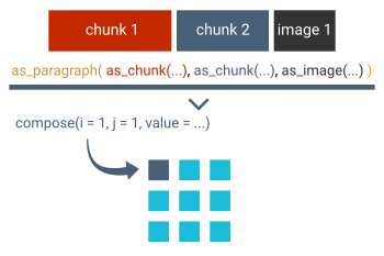
By default, the displayed content of each cell will be the result of a simple formatting. The content can also be composed as the result of a concatenation of several chunks.
The tables will all display cell contents representing the contents of the
corresponding input data.frame cell. If it’s a string, it will remain as is, if
it’s a number, it will be transformed into a string with a certain number of
decimal places, if it’s a date, it will be transformed into a string
representing a date, and so on.
The default display is conditioned by the type of data, i.e. columns of type
double will be formatted with colformat_double(), columns of type integer
will be formatted with colformat_int(), columns of type character will
be formatted with colformat_char() and so on.
First, we explain the use of the colformat_* functions and then we will see how to fill cells with richer contents (i.e. being able to mix images, text and hyperlinks) with the compose(as_paragraph()) functions. Function compose() also exists in the ‘purrr’ package which often causes issues. The identical function mk_par() has been created to avoid package conflict issues, i.e. flextable::mk_par() and flextable::compose() are the same exact functions. For clarity, only mk_par() is used in this book.
Before showing tables, let’s specify their post-processing before
printing with function autofit():
set_flextable_defaults(
  post_process_html = autofit,
  post_process_pdf = autofit,
  post_process_docx = autofit
  )
5.1 Soft returns and tabulations
A cell is made of one single paragraph of text. Paragraphs can contain several chunks of text with different formatting but also images. (See keypoints.)
When working with flextable, if a string contains \n or \t, it
will be treated as a soft return (not a new paragraph!) or a tabulation.
We don’t recommend changing your data so that it contains \n or \t. Instead
we recommend using mk_par(), prepend_chunks() or append_chunks(). See
[#multi-content] for more details about these functions.
dat <- data.frame(a = c("Grand total", letters[1:4]))
flextable(dat) |>
  prepend_chunks(i = ~ a != "Grand total", j = "a", as_chunk("\t"))
a |
|---|
Grand total |
a |
b |
c |
d |
5.1.1 Tab stops
When text contains \t, the position where the cursor jumps can be controlled
with tab_settings(). It uses officer::fp_tabs() and officer::fp_tab() to
define tab stop positions and styles (e.g. decimal alignment).
This is useful for clinical tables where numbers must be aligned on the decimal point. Tab stops only work with Word and RTF outputs.
library(officer)

dat <- data.frame(
  Statistic = c("Median (Q1 ; Q3)", "Min ; Max"),
  Value = c(
    "\t999.99\t(99.9 ; 99.9)",
    "\t9.99\t(9999.9 ; 99.9)"
  )
)

ts <- fp_tabs(
  fp_tab(pos = 0.4, style = "decimal"),
  fp_tab(pos = 1.4, style = "decimal")
)

ft <- flextable(dat) |>
  tab_settings(j = "Value", value = ts) |>
  width(width = c(1.5, 2))
save_as_docx(ft, path = "reports/tab_settings_example.docx")
5.2 Simple formatting of cell content
These are high level functions that should satisfy most of the usual formatting needs. They can be used to define the formatting of one or more columns and eventually on a subset of rows.
Each accepts a prefix and suffix argument that can be used
to add a currency symbol for example. Also they all have
a na_str argument (default to ““), the string to use when data
are not available.
-
colformat_num()let you format columns of type numeric as it is formatted in your R console. This is the default function applied to all numeric columns when a flextable is created. It does not supportdigitsargument, it uses default R options through calls toformat(). -
colformat_double()with argumentsdigitsandbig.mark: let you format columns of type double. -
colformat_int()with argumentsbig.mark: let you format columns of type integer. -
colformat_char(): let you format columns of type character. -
colformat_lgl(): let you format columns of type logical. -
colformat_image(): let you format image paths as images. -
colformat_date()andcolformat_datetime(): let you format columns of type date and datetime (POSIX).
The following illustration is using dataset “people” (see table B.4).
flextable(people) %>%
  colformat_num(
    big.mark = " ", decimal.mark = ",",
    na_str = "na") %>%
  colformat_int(big.mark = " ") %>%
  colformat_char(j = "eye_color", prefix = "color: ") %>%
  colformat_date(fmt_date = "%d/%m/%Y")
name |
birthday |
n_children |
weight |
height |
n_peanuts |
eye_color |
|---|---|---|---|---|---|---|
Olivier Gomes-Benard |
10/04/2030 |
4 |
70,08947 |
182,4731 |
1 030 700 |
color: blue |
Alexandrie Delaunay |
01/02/2008 |
0 |
na |
177,0763 |
1 028 912 |
color: blue |
Laure d'Dumont |
29/12/2017 |
4 |
na |
167,3393 |
1 197 083 |
color: dark |
Jean Pineau |
14/01/2038 |
1 |
na |
177,5332 |
933 946 |
color: dark |
Denis Pottier |
09/10/2023 |
4 |
79,72488 |
174,8449 |
918 810 |
color: green |
Éric L'Courtois |
11/07/1993 |
3 |
60,62562 |
165,6048 |
962 597 |
color: green |
Vincent Grondin |
26/04/2009 |
0 |
66,95984 |
160,6060 |
1 119 724 |
color: dark |
Roland Navarro |
20/08/2014 |
1 |
80,96033 |
168,6873 |
563 028 |
color: dark |
Clémence Morél |
23/08/2022 |
4 |
56,37211 |
169,2335 |
817 860 |
color: green |
Anne Faivre |
29/07/2023 |
3 |
51,62123 |
168,4341 |
563 869 |
color: dark |
Keep in mind that by setting the default display values, these calls can be avoided in most cases. They can be updated with function set_flextable_defaults().
old_settings <- set_flextable_defaults(
  digits = 1, decimal.mark = ",", big.mark = " ",
  na_str = "na", fmt_date = "%d/%m/%Y")

flextable(people)
name |
birthday |
n_children |
weight |
height |
n_peanuts |
eye_color |
|---|---|---|---|---|---|---|
Olivier Gomes-Benard |
10/04/2030 |
4 |
70,08947 |
182,4731 |
1 030 700 |
blue |
Alexandrie Delaunay |
01/02/2008 |
0 |
na |
177,0763 |
1 028 912 |
blue |
Laure d'Dumont |
29/12/2017 |
4 |
na |
167,3393 |
1 197 083 |
dark |
Jean Pineau |
14/01/2038 |
1 |
na |
177,5332 |
933 946 |
dark |
Denis Pottier |
09/10/2023 |
4 |
79,72488 |
174,8449 |
918 810 |
green |
Éric L'Courtois |
11/07/1993 |
3 |
60,62562 |
165,6048 |
962 597 |
green |
Vincent Grondin |
26/04/2009 |
0 |
66,95984 |
160,6060 |
1 119 724 |
dark |
Roland Navarro |
20/08/2014 |
1 |
80,96033 |
168,6873 |
563 028 |
dark |
Clémence Morél |
23/08/2022 |
4 |
56,37211 |
169,2335 |
817 860 |
green |
Anne Faivre |
29/07/2023 |
3 |
51,62123 |
168,4341 |
563 869 |
dark |
do.call(set_flextable_defaults, old_settings)5.3 Replace displayed labels
The function labelizor() replaces text values in a flextable with labels. The labels are defined with character named vector or with a function that transforms the existing text.
Let’s illustrate these two options with a table representing an aggregation.
library(palmerpenguins)

ft_pen <- penguins |>
  select(species, island, ends_with("mm")) |>
  group_by(species, island) |>
  summarise(
    across(
      where(is.numeric),
      .fns = list(
        avg = ~ mean(.x, na.rm = TRUE),
        sd = ~ sd(.x, na.rm = TRUE)
      )
    ),
    .groups = "drop") |>
  rename_with(~ tolower(gsub("_mm_", "_", .x, fixed = TRUE))) |>
  flextable() |>
  colformat_double() |>
  separate_header() |>
  theme_vanilla() |>
  align(align = "center", part = "all") |>
  valign(valign = "center", part = "header") |>
  autofit()
ft_pen
species |
island |
bill |
flipper |
||||
|---|---|---|---|---|---|---|---|
length |
depth |
length |
|||||
avg |
sd |
avg |
sd |
avg |
sd |
||
Adelie |
Biscoe |
39.0 |
2.5 |
18.4 |
1.2 |
188.8 |
6.7 |
Adelie |
Dream |
38.5 |
2.5 |
18.3 |
1.1 |
189.7 |
6.6 |
Adelie |
Torgersen |
39.0 |
3.0 |
18.4 |
1.3 |
191.2 |
6.2 |
Chinstrap |
Dream |
48.8 |
3.3 |
18.4 |
1.1 |
195.8 |
7.1 |
Gentoo |
Biscoe |
47.5 |
3.1 |
15.0 |
1.0 |
217.2 |
6.5 |
Now, let’s replace the names of calculated columns with prettier labels:
ft_pen <- labelizor(
  x = ft_pen,
  part = "header",
  labels = c("avg" = "Mean", "sd" = "Standard Deviation"))
ft_pen
species |
island |
bill |
flipper |
||||
|---|---|---|---|---|---|---|---|
length |
depth |
length |
|||||
Mean |
Standard Deviation |
Mean |
Standard Deviation |
Mean |
Standard Deviation |
||
Adelie |
Biscoe |
39.0 |
2.5 |
18.4 |
1.2 |
188.8 |
6.7 |
Adelie |
Dream |
38.5 |
2.5 |
18.3 |
1.1 |
189.7 |
6.6 |
Adelie |
Torgersen |
39.0 |
3.0 |
18.4 |
1.3 |
191.2 |
6.2 |
Chinstrap |
Dream |
48.8 |
3.3 |
18.4 |
1.1 |
195.8 |
7.1 |
Gentoo |
Biscoe |
47.5 |
3.1 |
15.0 |
1.0 |
217.2 |
6.5 |
And now, let’s format headers with title case:
ft_pen <- labelizor(
  x = ft_pen,
  part = "header",
  labels = stringr::str_to_title)
ft_pen
Species |
Island |
Bill |
Flipper |
||||
|---|---|---|---|---|---|---|---|
Length |
Depth |
Length |
|||||
Mean |
Standard Deviation |
Mean |
Standard Deviation |
Mean |
Standard Deviation |
||
Adelie |
Biscoe |
39.0 |
2.5 |
18.4 |
1.2 |
188.8 |
6.7 |
Adelie |
Dream |
38.5 |
2.5 |
18.3 |
1.1 |
189.7 |
6.6 |
Adelie |
Torgersen |
39.0 |
3.0 |
18.4 |
1.3 |
191.2 |
6.2 |
Chinstrap |
Dream |
48.8 |
3.3 |
18.4 |
1.1 |
195.8 |
7.1 |
Gentoo |
Biscoe |
47.5 |
3.1 |
15.0 |
1.0 |
217.2 |
6.5 |
5.4 Multi content
The user can have more control over displayed content by using function
compose() or mk_par() which are identical. The function enables the user to define the elements composing the paragraph
and their respective formats. It can also be used to mix text chunks and images.
5.4.1 Function mk_par
flextable content can be defined with function mk_par().
It lets the user control the formatted content at the cell level of the table. It is possible to define content for a row subset and a column as well as for the whole column. One can mix images and text (but not with PowerPoint because PowerPoint cannot do it).
The function requires a call to as_paragraph() which will
concatenate text or images chunks as a paragraph.
The following illustration is using dataset “fishes” (see table B.3). It shows how to control the format of displayed values and how to associate them with specific text formatting properties:
ft <- flextable(fishes) %>%
  mk_par(j = "latin_name",
          value = as_paragraph(
            as_chunk(latin_name,
                     props = fp_text_default(color = "#C32900", bold = TRUE)))) %>%
  mk_par(j = "french_name",
          value = as_paragraph(
            as_chunk(french_name,
                     props = fp_text_default(color = "#006699", bold = TRUE))))
ft
latin_name |
french_name |
X00 |
X01 |
|---|---|---|---|
Acipenser Sturio |
(L. 1758) Esturgeon européen |
||
Alosa alosa |
(L.1758) Alose vraie |
+ |
+ |
Alosa fallax |
(Lac. 1803) Alose feinte |
+ |
+ |
Anguilla anguilla |
(L. 1758) Anguille |
+ |
+ |
Lampetra fluviatilis |
(L. 1758) Lamproie de rivière |
+ |
|
Liza ramada |
(Risso 1826) Mulet porc |
+ |
+ |
With this system, it’s easy to concatenate multiple values:
ft <- flextable(fishes, col_keys = c("dummy", "X00", "X01")) %>%
  mk_par(j = "dummy", value = as_paragraph(as_i(latin_name), as_b(french_name))) %>%
  color(j = "dummy", color = "#006699") %>%
  set_header_labels(dummy = "Species")
ft
Species |
X00 |
X01 |
|---|---|---|
Acipenser Sturio (L. 1758) Esturgeon européen |
||
Alosa alosa (L.1758) Alose vraie |
+ |
+ |
Alosa fallax (Lac. 1803) Alose feinte |
+ |
+ |
Anguilla anguilla (L. 1758) Anguille |
+ |
+ |
Lampetra fluviatilis (L. 1758) Lamproie de rivière |
+ |
|
Liza ramada (Risso 1826) Mulet porc |
+ |
+ |
Or to define specific title headers:
mk_par(
  ft, j = "dummy", part = "header",
  value = as_paragraph(
    "Species ",
    as_chunk("* latin/french name",
             props = fp_text_default(color = "#006699", vertical.align = "superscript"))
    )
  )
Species * latin/french name |
X00 |
X01 |
|---|---|---|
Acipenser Sturio (L. 1758) Esturgeon européen |
||
Alosa alosa (L.1758) Alose vraie |
+ |
+ |
Alosa fallax (Lac. 1803) Alose feinte |
+ |
+ |
Anguilla anguilla (L. 1758) Anguille |
+ |
+ |
Lampetra fluviatilis (L. 1758) Lamproie de rivière |
+ |
|
Liza ramada (Risso 1826) Mulet porc |
+ |
+ |
Note that mk_par is not appending but is replacing the content.
5.4.2 Sugar functions for complex formatting
Functions as_b, as_i, as_sub, as_sup and as_strike are special
functions that can be used together. They set a value as bold, italic,
subscripted, superscripted or struck through (strikethrough).
This is particularly useful when the headers need complex formatting.
data <- structure(list(Species = structure(1:3, .Label = c("setosa",
"versicolor", "virginica"), class = "factor"), col1 = c(5.006,
5.936, 6.588)), class = "data.frame", row.names = c(NA, -3L))

ft <- flextable(data) %>%
  mk_par(
    part = "header", j = "Species",
    value = as_paragraph(as_i(as_b("Species")))
  ) %>%
  mk_par(
    part = "header", j = "col1",
    value = as_paragraph(as_b("µ"), as_sup("blah"))
  )
ft
Species |
µblah |
|---|---|
setosa |
5.006 |
versicolor |
5.936 |
virginica |
6.588 |
as_strike() applies strikethrough formatting; it can also be applied to
the whole text with the fp_text_default(strike = TRUE) property.
flextable(head(iris, 3), col_keys = c("Sepal.Length", "dummy")) %>%
  mk_par(
    j = "dummy",
    value = as_paragraph(as_strike(Sepal.Length))
  )
Sepal.Length |
|
|---|---|
5.1 |
5.1 |
4.9 |
4.9 |
4.7 |
4.7 |
5.4.3 Append or prepend content
prepend_chunks() or append_chunks() functions are handy functions that
let users add in an existing paragraph one or more chunks. It can be any
function dedicated to chunk creation, i.e. as_image(), as_chunk(),
as_equation(), gg_chunk(), plot_chunk(). Function prepend_chunks()
can be used to add tabulations for example.
ft <- flextable(data) %>%
  append_chunks(
    part = "body", i = 1, j = "Species",
    as_b(" some bold text")
  ) %>%
  prepend_chunks(
    part = "body", j = "col1", i = 2,
    as_chunk("hello ", props = fp_text_default(color = "red"))
  )
ft
Species |
col1 |
|---|---|
setosa some bold text |
5.006 |
versicolor |
hello 5.936 |
virginica |
6.588 |
5.5 Images
Function mk_par supports image insertion. Use function as_image in
as_paragraph call.
The following illustration is using dataset “Tennis players” (see table B.1).
To display only one image per cell, you can use the colformat_image function.
The dimensions of the image(s) must always be specified.
flextable(tennis_players) %>%
  colformat_image(j = "head", width = .5, height = 0.5) %>%
  colformat_image(j = "flag", width = .5, height = 0.33)
Rank |
Player |
Percentage |
Games.Won |
Total.Games |
Matches |
head |
flag |
|---|---|---|---|---|---|---|---|
1 |
Roger Federer |
92.63 |
2 739 |
2 957 |
205 |
|
|
2 |
Lleyton Hewitt |
85.29 |
1 740 |
2 040 |
149 |
|
|
3 |
Feliciano Lopez |
89.86 |
1 684 |
1 874 |
122 |
|
|
4 |
Ivo Karlovic |
94.87 |
1 645 |
1 734 |
113 |
|
|
5 |
Andy Murray |
88.89 |
1 528 |
1 719 |
121 |
|
|
6 |
Pete Sampras |
92.66 |
1 478 |
1 595 |
105 |
|
|
7 |
Greg Rusedski |
90.33 |
1 476 |
1 634 |
116 |
|
|
8 |
Tim Henman |
83.77 |
1 461 |
1 744 |
110 |
|
|
9 |
Novak Djokovic |
89.12 |
1 442 |
1 618 |
106 |
|
|
10 |
Andy Roddick |
92.76 |
1 410 |
1 520 |
103 |
|
|


For a more complex display, such as mixing text and image,
use the mk_par and as_image functions.
flextable(tennis_players,
  col_keys = c(
    "Rank", "Player", "Percentage",
    "Games.Won", "Total.Games", "Matches"
  )
) %>%
  mk_par(
    j = "Player",
    value = as_paragraph(
      as_image(src = head, width = .5, height = 0.5),
      " ",
      as_image(src = flag, width = .5, height = 0.33),
      " ", as_chunk(x = Player, fp_text_default(color = "#337ab7"))
    )
  )
Rank |
Player |
Percentage |
Games.Won |
Total.Games |
Matches |
|---|---|---|---|---|---|
1 |
|
92.63 |
2 739 |
2 957 |
205 |
2 |
|
85.29 |
1 740 |
2 040 |
149 |
3 |
|
89.86 |
1 684 |
1 874 |
122 |
4 |
|
94.87 |
1 645 |
1 734 |
113 |
5 |
|
88.89 |
1 528 |
1 719 |
121 |
6 |
|
92.66 |
1 478 |
1 595 |
105 |
7 |
|
90.33 |
1 476 |
1 634 |
116 |
8 |
|
83.77 |
1 461 |
1 744 |
110 |
9 |
|
89.12 |
1 442 |
1 618 |
106 |
10 |
|
92.76 |
1 410 |
1 520 |
103 |
5.6 Images and limitations of PowerPoint
Using images in flextable is not supported when the output format is PowerPoint. This is not a choice nor an unimplemented feature. This is because PowerPoint is not able to embed images in a table cell. That’s a PowerPoint limitation. The same limitation occurs with ggplot charts and mini charts.
If being able to display images in PowerPoint tables is important to you, you
can use the plot function or the save_as_image and embed the result in the
PowerPoint. You will of course lose the ability to edit the table in PowerPoint.
5.7 Mini charts
set_flextable_defaults(
  post_process_html = function(x){
    theme_alafoli(x) %>%
      align(align = "center", part = "all") %>%
      align(align = "left", part = "footer") %>%
      autofit()
  }
)
5.7.1 base plots and ggplot objects
There are four types of mini plots available that can be inserted into flextables: ‘box’, ‘line’, ‘points’ and
‘density’. This requires storing a list column in your data.frame as these
are functions that need more than a single point.
z <- as.data.table(iris)
z <- z[, list(
  data = list(.SD$Sepal.Length)
), by = "Species"]

flextable(z) %>%
  mk_par(j = "data", value = as_paragraph(
    plot_chunk(value = data, type = "dens", col = "red")
    ))
Species |
data |
|---|---|
setosa |
|
versicolor |
|
virginica |
|


ggplot objects are supported and can be inserted with gg_chunk(). It lets users implement
any graphics with ggplot2.
It usually requires a structure containing data grouped by one or more
factors and a function to
call on each content that produces a ggplot graph (in which
adding the theme_void() is common).
Below, the function used to draw bars:
gg_bars <- function(z) {
  z <- scale(z)
  z <- na.omit(z)
  z <- data.frame(x = seq_along(z), z = z, w = z < 0)
  ggplot(z, aes(x = x, y = z, fill = w)) +
    geom_col(show.legend = FALSE) +
    theme_void()
}
Now the dataset:
dat <- as.data.table(mtcars)
z <- dat[,
  lapply(.SD, function(x) list(gg_bars(x))),
  by = c("vs", "am"), .SDcols = c("mpg", "disp", "drat")
]
And now the flextable with the ggplots:
ft <- flextable(z)
ft <- mk_par(ft,
    j = c("mpg", "disp", "drat"),
    value = as_paragraph(gg_chunk(value = ., height = .15, width = 1)),
    use_dot = TRUE
  )
ft
vs |
am |
mpg |
disp |
drat |
|---|---|---|---|---|
0 |
1 |
|
|
|
1 |
1 |
|
|
|
1 |
0 |
|
|
|
0 |
0 |
|
|
|


5.7.2 minibar
Function mk_par supports mini barplots insertion. Use function
minibar in as_paragraph call:
flextable( head(iris, n = 10 )) %>%
  mk_par(j = 1,
          value = as_paragraph(
            minibar(value = Sepal.Length, max = max(Sepal.Length), height = .15)
            ),
  part = "body")
Sepal.Length |
Sepal.Width |
Petal.Length |
Petal.Width |
Species |
|---|---|---|---|---|
|
3.5 |
1.4 |
0.2 |
setosa |
|
3.0 |
1.4 |
0.2 |
setosa |
|
3.2 |
1.3 |
0.2 |
setosa |
|
3.1 |
1.5 |
0.2 |
setosa |
|
3.6 |
1.4 |
0.2 |
setosa |
|
3.9 |
1.7 |
0.4 |
setosa |
|
3.4 |
1.4 |
0.3 |
setosa |
|
3.4 |
1.5 |
0.2 |
setosa |
|
2.9 |
1.4 |
0.2 |
setosa |
|
3.1 |
1.5 |
0.1 |
setosa |


5.7.3 linerange
Function mk_par supports mini linerange insertion. Use function linerange in as_paragraph call:
flextable( head(iris, n = 10 )) %>%
  mk_par(j = 1,
          value = as_paragraph(
            linerange(value = Sepal.Length, max = max(Sepal.Length), height = .15)
            ),
  part = "body")
Sepal.Length |
Sepal.Width |
Petal.Length |
Petal.Width |
Species |
|---|---|---|---|---|
|
3.5 |
1.4 |
0.2 |
setosa |
|
3.0 |
1.4 |
0.2 |
setosa |
|
3.2 |
1.3 |
0.2 |
setosa |
|
3.1 |
1.5 |
0.2 |
setosa |
|
3.6 |
1.4 |
0.2 |
setosa |
|
3.9 |
1.7 |
0.4 |
setosa |
|
3.4 |
1.4 |
0.3 |
setosa |
|
3.4 |
1.5 |
0.2 |
setosa |
|
2.9 |
1.4 |
0.2 |
setosa |
|
3.1 |
1.5 |
0.1 |
setosa |


