Chapter 12 Plotting flextable

wrap_flextable() wraps a flextable as a patchwork-compliant patch. It allows flextable objects to be combined with ggplot2 plots using the +, |, and / operators from patchwork.

To illustrate, we build a dumbbell chart of Bundesliga team statistics paired with a matching flextable (adapted from the R Graph Gallery).

library(ggplot2)
library(patchwork)

dataset <- data.frame(
  team = c(
    "FC Bayern Munchen", "SV Werder Bremen", "Borussia Dortmund",
    "VfB Stuttgart", "Borussia M'gladbach", "Hamburger SV",
    "Eintracht Frankfurt", "FC Schalke 04", "1. FC Koln",
    "Bayer 04 Leverkusen"
  ),
  matches = c(2000, 1992, 1924, 1924, 1898, 1866, 1856, 1832, 1754, 1524),
  won     = c(1206,  818,  881,  782,  763,  746,  683,  700,  674,  669),
  lost    = c( 363,  676,  563,  673,  636,  625,  693,  669,  628,  447)
)
dataset$win_pct  <- dataset$won  / dataset$matches * 100
dataset$loss_pct <- dataset$lost / dataset$matches * 100
dataset$team <- factor(dataset$team, levels = rev(dataset$team))

The dumbbell chart:

pal <- c(lost = "#EFAC00", won = "#28A87D")
df_long <- reshape(dataset, direction = "long",
  varying = list(c("loss_pct", "win_pct")),
  v.names = "pct", timevar = "type",
  times = c("lost", "won"), idvar = "team"
)

p <- ggplot(df_long, aes(x = pct / 100, y = team)) +
  stat_summary(
    geom = "linerange", fun.min = "min", fun.max = "max",
    linewidth = .7, color = "grey60"
  ) +
  geom_point(aes(fill = type), size = 4, shape = 21,
    stroke = .8, color = "white"
  ) +
  scale_x_continuous(
    labels = scales::percent,
    expand = expansion(add = c(.02, .02))
  ) +
  scale_y_discrete(name = NULL, guide = "none") +
  scale_fill_manual(
    values = pal,
    labels = c(lost = "Lost", won = "Won")
  ) +
  labs(x = NULL, fill = NULL) +
  theme_minimal(base_size = 10) +
  theme(
    legend.position = "top",
    legend.justification = "left",
    panel.grid.minor = element_blank(),
    panel.grid.major.y = element_blank()
  )
p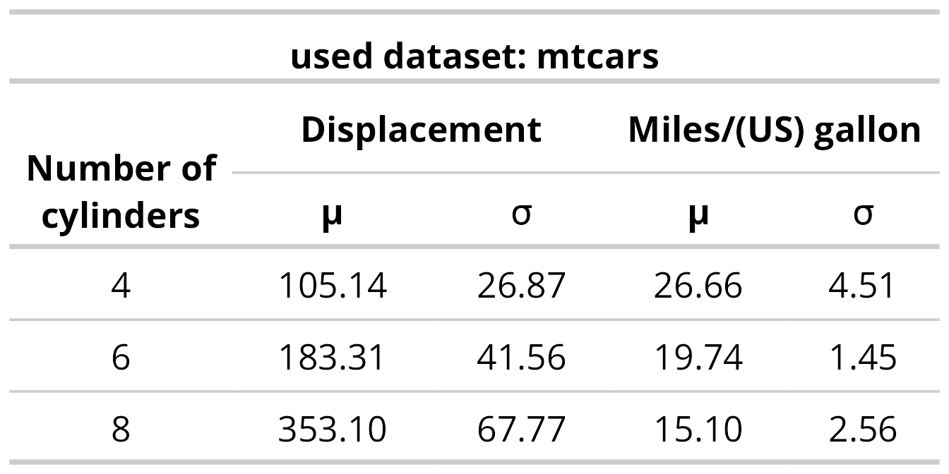

And the flextable:

ft_dat <- dataset[, c("matches", "win_pct", "loss_pct", "team")]
ft_dat$team <- as.character(ft_dat$team)

ft <- flextable(ft_dat) |>
  border_remove() |>
  bold(part = "header") |>
  colformat_double(j = c("win_pct", "loss_pct"),
    digits = 1, suffix = "%") |>
  set_header_labels(
    team = "Team", matches = "GP",
    win_pct = "Won", loss_pct = "Lost") |>
  color(color = "#28A87D", j = "win_pct") |>
  color(color = "#EFAC00", j = "loss_pct") |>
  bold(j = c("win_pct", "loss_pct")) |>
  italic(j = "team") |>
  align(align = "right", part = "all") |>
  autofit()
ft

GP	Won	Lost	Team
2 000	60.3%	18.1%	FC Bayern Munchen
1 992	41.1%	33.9%	SV Werder Bremen
1 924	45.8%	29.3%	Borussia Dortmund
1 924	40.6%	35.0%	VfB Stuttgart
1 898	40.2%	33.5%	Borussia M'gladbach
1 866	40.0%	33.5%	Hamburger SV
1 856	36.8%	37.3%	Eintracht Frankfurt
1 832	38.2%	36.5%	FC Schalke 04
1 754	38.4%	35.8%	1. FC Koln
1 524	43.9%	29.3%	Bayer 04 Leverkusen

12.1 Basic usage

Use wrap_flextable() to place a flextable alongside ggplot2 plots.

wrap_flextable(ft) | p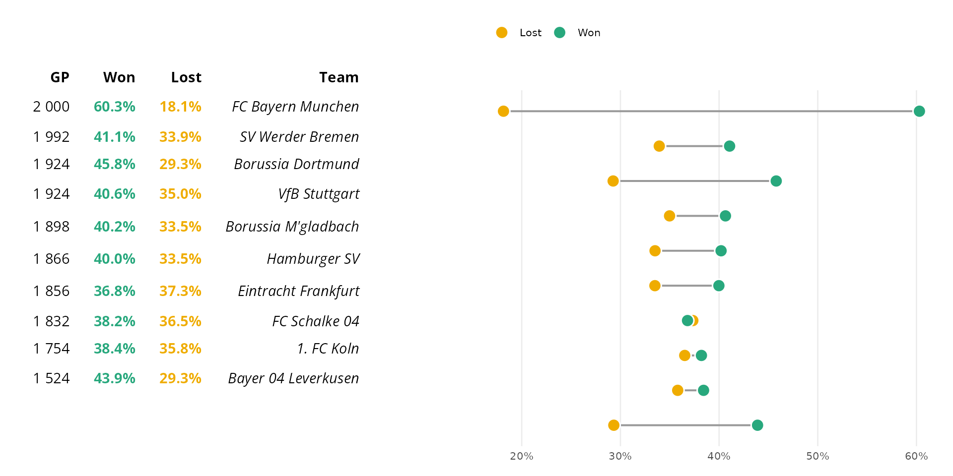

12.2 Aligning rows with `flex_body`

When flex_body = TRUE, body rows stretch to match the height of the adjacent plot panel. Each table row aligns with the corresponding category on the y axis. Header and footer keep their fixed size.

wrap_flextable(ft, flex_body = TRUE, just = "right") +
  p +
  plot_layout(widths = c(1.1, 2))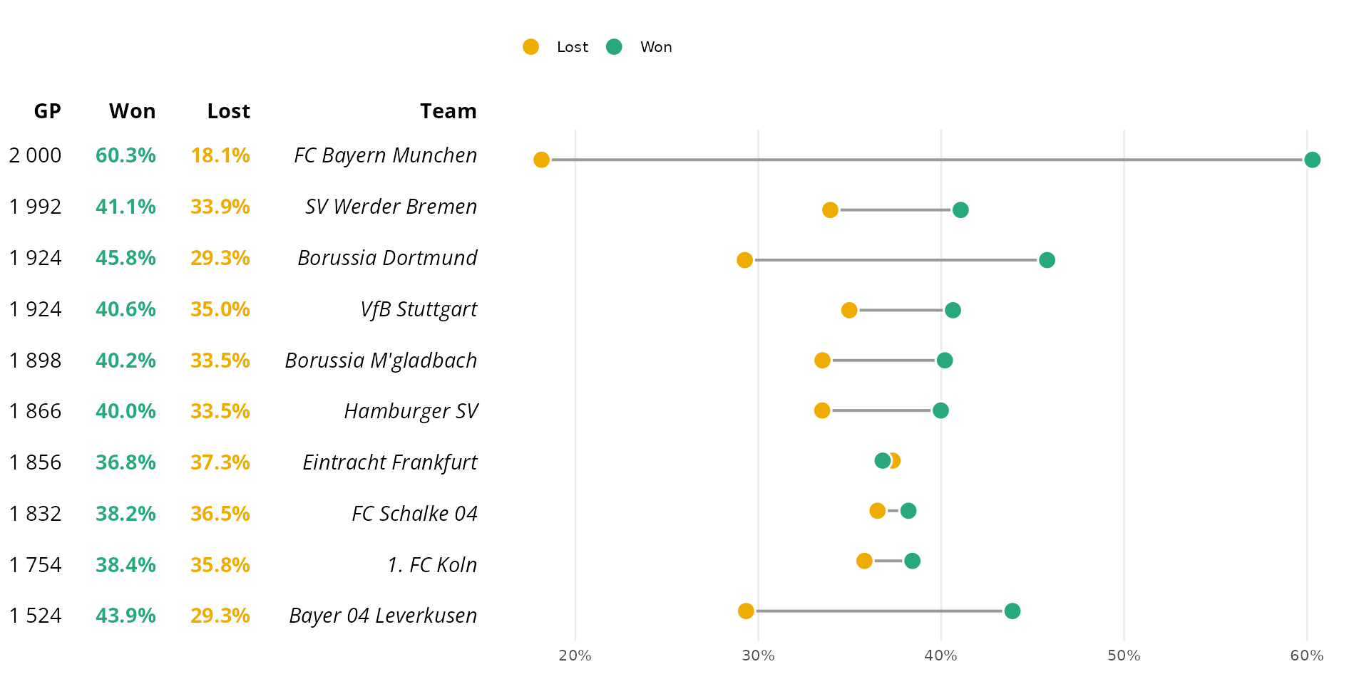

12.3 Aligning columns with `flex_cols`

When flex_cols = TRUE, data columns stretch to fill the panel width determined by the adjacent plot. Each column aligns with the corresponding category on the x axis. Use n_row_headers to exclude leading columns from stretching.

cyl_mpg <- aggregate(mpg ~ cyl, mtcars, mean)

gg_bar <- ggplot(cyl_mpg, aes(factor(cyl), mpg)) +
  geom_col(fill = "#28A87D", width = 0.7) +
  labs(x = "Cylinders", y = "Mean MPG") +
  theme_minimal(base_size = 10)

wide <- data.frame(t(round(cyl_mpg$mpg, 1)))
names(wide) <- cyl_mpg$cyl

ft_cyl <- flextable(wide) |>
  bold(part = "header") |>
  align(align = "center", part = "all") |>
  autofit()

wrap_flextable(ft_cyl, flex_cols = TRUE) /
  gg_bar +
  plot_layout(heights = c(1, 4))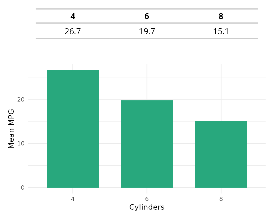

12.4 Horizontal alignment with `just`

The just argument controls horizontal alignment of the table within its patchwork panel: "left" (default), "right", or "center".

wrap_flextable(ft, just = "left") | p

wrap_flextable(ft, just = "right") | p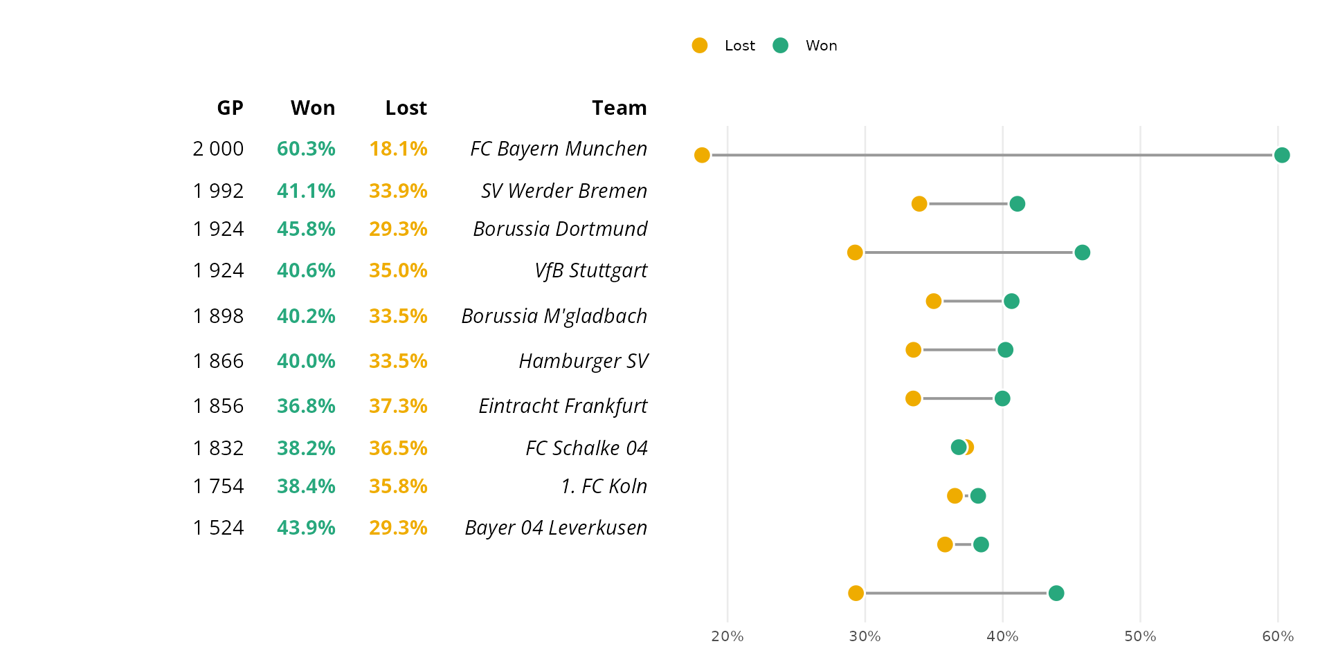

12.5 Panel alignment

The panel argument controls what portion of the table aligns with the plot panel region:

"body" (default): header and footer fall outside the panel region.
"full": the whole table is placed inside the panel region.

wrap_flextable(ft, panel = "body", flex_body = TRUE, just = "right") +
  p +
  plot_layout(widths = c(1.1, 2))

wrap_flextable(ft, panel = "full", flex_body = TRUE, just = "right") +
  p +
  plot_layout(widths = c(1.1, 2))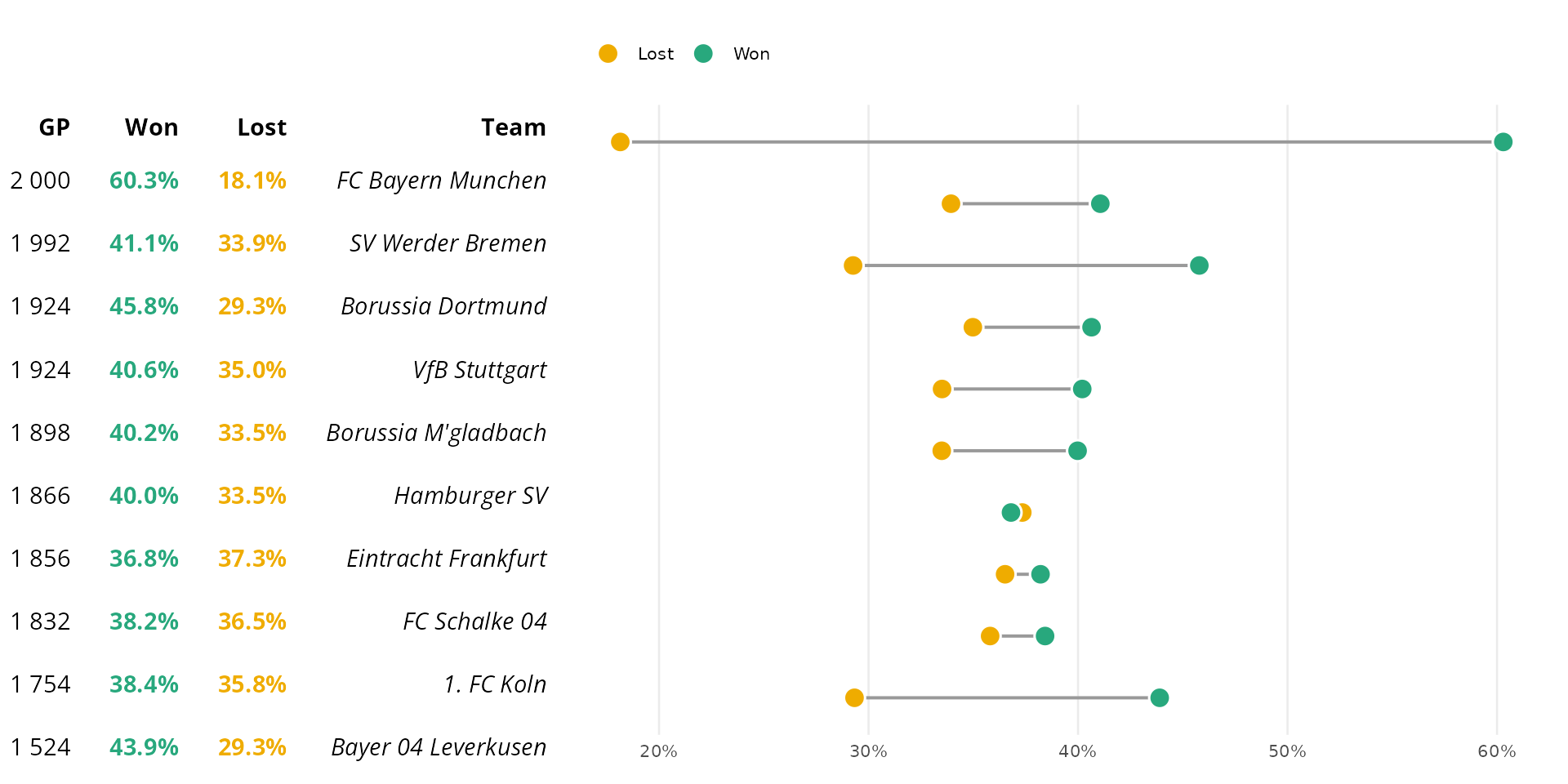

12.6 Saving as image

Use save_as_image() to export a flextable as a PNG or SVG file:

save_as_image(ft, path = "table.png")
save_as_image(ft, path = "table.svg")