Chapter 3 Table design

3.1 Table parts

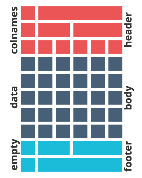
A flextable object is composed of 3 parts:

• header: by default there is only one header row containing the names of the data.frame.
• body: by default contains the data from the data.frame.
• footer: none by default but can contain content. Commonly used for footnotes.

ft <- flextable(head(airquality))
ft

Table 3.1: default flextable

Ozone	Solar.R	Wind	Temp	Month	Day
41	190	7.4	67	5	1
36	118	8.0	72	5	2
12	149	12.6	74	5	3
18	313	11.5	62	5	4
<na>	<na>	14.3	56	5	5
28	<na>	14.9	66	5	6

The parts can be augmented with new lines.

ft <- add_header_row(ft, values = c("air quality", "time"), colwidths = c(4, 2))
ft <- add_footer_lines(ft, "hello note")
ft

Table 3.2: default flextable with headers and a footer

air quality				time
Ozone	Solar.R	Wind	Temp	Month	Day
41	190	7.4	67	5	1
36	118	8.0	72	5	2
12	149	12.6	74	5	3
18	313	11.5	62	5	4
<na>	<na>	14.3	56	5	5
28	<na>	14.9	66	5	6
hello note

3.2 Visible columns

A flextable is an object that produces a reporting table from a data.frame object.

Parameter col_keys of function flextable defines which dataset variables to show and their order. Visible columns are by default all columns of the dataset.

myft <- flextable(
  data = head(airquality), 
  col_keys = c("Ozone", "Solar.R", "Wind", "Temp", 
               "Month", "Day"))
myft

Ozone	Solar.R	Wind	Temp	Month	Day
41	190	7.4	67	5	1
36	118	8.0	72	5	2
12	149	12.6	74	5	3
18	313	11.5	62	5	4
<na>	<na>	14.3	56	5	5
28	<na>	14.9	66	5	6

Dataset variables can be chosen from existing columns but also non-existent columns. When a value of parameter col_keys has a name that does not exist in the dataset, it is considered as a blank column with no data mapping.

These blank columns can be used as separators. Non-existent columns contain empty string values ("") for each row by default.

myft <- flextable(
  data = head(airquality), 
  col_keys = c("Ozone", "Solar.R", "col1", "Month", "Day")) |> 
  width(j = "col1", width = .2) |> 
  empty_blanks()
myft

Ozone	Solar.R		Month	Day
41	190		5	1
36	118		5	2
12	149		5	3
18	313		5	4
<na>	<na>		5	5
28	<na>		5	6

Non-existant column values can be defined with functions such as mk_par() or append_chunks().

The following example shows how to highlight some rows according to a condition; if the condition is TRUE, colored text is added in the blank column.

library(grid)
myft |> 
  append_chunks(
    i = ~ Ozone < 30, j = "col1", 
    as_chunk(";)", props = fp_text_default(color = "#ec11c2")))

Ozone	Solar.R		Month	Day
41	190		5	1
36	118		5	2
12	149	;)	5	3
18	313	;)	5	4
<na>	<na>		5	5
28	<na>	;)	5	6

By default, the cells are filled with the content of the data.frame cells, the values are formatted with the function format. The displayed content of the cells can be updated, i.e. you can define the decimal separator, the text representing missing values, a text to be used as a suffix or prefix.

With flextable, a cell is made of one single paragraph of text. Paragraphs can contain several chunks of text with different formatting but also images and equations. It is possible to create composite content, i.e. composed of several pieces of text, images and even ggplot graphics.

# data prep ----
z <- as.data.table(ggplot2::diamonds)
z <- z[, list(
  price = mean(price, na.rm = TRUE),
  list_col = list(.SD$x)
), by = "cut"]

# flextable ----
ft <- flextable(data = z) %>%
  mk_par(j = "list_col", value = as_paragraph(
    plot_chunk(value = list_col, type = "dens", col = "#ec11c2", 
               width = 1.5, height = .4, free_scale = TRUE)
  )) %>%
  colformat_double(big.mark = " ", suffix = " $") %>% 
  autofit()
ft

Table 3.3: mixing text and plots

cut	price	list_col
Ideal	3 457.54 $
Premium	4 584.26 $
Good	3 928.86 $
Very Good	3 981.76 $
Fair	4 358.76 $

3.3 Selectors

Selectors can be used to specify the rows and columns where an operation should happened. Many flextable functions have selectors i and j: bg(), bold(), hline(), color(), padding(), fontsize(), italic(), align(), compose().

It makes conditional formatting easy and multiple operations can be seamlessly piped (with magrittr::%>% or |>).

dat <- head(ggplot2::diamonds, n = 10)
qflextable(dat) %>% 
  color(~ price < 330, color = "orange", ~ price + x + y + z ) %>% 
  color(~ carat > .24, ~ cut, color = "red")

carat	cut	color	clarity	depth	table	price	x	y	z
0.23	Ideal	E	SI2	61.5	55	326	3.95	3.98	2.43
0.21	Premium	E	SI1	59.8	61	326	3.89	3.84	2.31
0.23	Good	E	VS1	56.9	65	327	4.05	4.07	2.31
0.29	Premium	I	VS2	62.4	58	334	4.20	4.23	2.63
0.31	Good	J	SI2	63.3	58	335	4.34	4.35	2.75
0.24	Very Good	J	VVS2	62.8	57	336	3.94	3.96	2.48
0.24	Very Good	I	VVS1	62.3	57	336	3.95	3.98	2.47
0.26	Very Good	H	SI1	61.9	55	337	4.07	4.11	2.53
0.22	Fair	E	VS2	65.1	61	337	3.87	3.78	2.49
0.23	Very Good	H	VS1	59.4	61	338	4.00	4.05	2.39

Default values for i and j are NULL, NULL value is interpreted as all rows or all columns.

3.3.1 Usage

i for rows selection and j for columns selection can be expressed in different ways:

3.3.1.1 as a formula

Use i = ~ col %in% "xxx" to select all rows where values from column ‘col’ are “xxx”.

The argument expression is ~ and then an R expression. There is no need to quote variable, when the formula is evaluated, values from the corresponding dataset (to the part) will be used.

To express multiple conditions, use operator & or |:

i = ~ col1 < 5 & col2 %in% "zzz"

The columns can also be selected with a formula. Use the + operator to select multiple columns. For example, to select columns col1 and col2: j = ~ col1 + col2

ft <- qflextable(dat)

color(
  ft, i = ~ cut %in% "Premium", 
  j = ~ x + y, color = "red")

carat	cut	color	clarity	depth	table	price	x	y	z
0.23	Ideal	E	SI2	61.5	55	326	3.95	3.98	2.43
0.21	Premium	E	SI1	59.8	61	326	3.89	3.84	2.31
0.23	Good	E	VS1	56.9	65	327	4.05	4.07	2.31
0.29	Premium	I	VS2	62.4	58	334	4.20	4.23	2.63
0.31	Good	J	SI2	63.3	58	335	4.34	4.35	2.75
0.24	Very Good	J	VVS2	62.8	57	336	3.94	3.96	2.48
0.24	Very Good	I	VVS1	62.3	57	336	3.95	3.98	2.47
0.26	Very Good	H	SI1	61.9	55	337	4.07	4.11	2.53
0.22	Fair	E	VS2	65.1	61	337	3.87	3.78	2.49
0.23	Very Good	H	VS1	59.4	61	338	4.00	4.05	2.39

3.3.1.2 as a character vector

Argument j supports simple character vectors containing the col_key names.

ft %>% 
  color(j = c("x", "y"), color = "orange", part = "all") %>% 
  bold(j = c("price", "x"), bold = TRUE)

carat	cut	color	clarity	depth	table	price	x	y	z
0.23	Ideal	E	SI2	61.5	55	326	3.95	3.98	2.43
0.21	Premium	E	SI1	59.8	61	326	3.89	3.84	2.31
0.23	Good	E	VS1	56.9	65	327	4.05	4.07	2.31
0.29	Premium	I	VS2	62.4	58	334	4.20	4.23	2.63
0.31	Good	J	SI2	63.3	58	335	4.34	4.35	2.75
0.24	Very Good	J	VVS2	62.8	57	336	3.94	3.96	2.48
0.24	Very Good	I	VVS1	62.3	57	336	3.95	3.98	2.47
0.26	Very Good	H	SI1	61.9	55	337	4.07	4.11	2.53
0.22	Fair	E	VS2	65.1	61	337	3.87	3.78	2.49
0.23	Very Good	H	VS1	59.4	61	338	4.00	4.05	2.39

3.3.1.3 as a integer vector

Each element is the row number or col_key number:

color(ft, i = 1:3, j = 1:3, color = "orange")

carat	cut	color	clarity	depth	table	price	x	y	z
0.23	Ideal	E	SI2	61.5	55	326	3.95	3.98	2.43
0.21	Premium	E	SI1	59.8	61	326	3.89	3.84	2.31
0.23	Good	E	VS1	56.9	65	327	4.05	4.07	2.31
0.29	Premium	I	VS2	62.4	58	334	4.20	4.23	2.63
0.31	Good	J	SI2	63.3	58	335	4.34	4.35	2.75
0.24	Very Good	J	VVS2	62.8	57	336	3.94	3.96	2.48
0.24	Very Good	I	VVS1	62.3	57	336	3.95	3.98	2.47
0.26	Very Good	H	SI1	61.9	55	337	4.07	4.11	2.53
0.22	Fair	E	VS2	65.1	61	337	3.87	3.78	2.49
0.23	Very Good	H	VS1	59.4	61	338	4.00	4.05	2.39

3.3.1.4 as a logical vector

color(ft, i = rep(c(TRUE, FALSE), 5), color = "orange")

carat	cut	color	clarity	depth	table	price	x	y	z
0.23	Ideal	E	SI2	61.5	55	326	3.95	3.98	2.43
0.21	Premium	E	SI1	59.8	61	326	3.89	3.84	2.31
0.23	Good	E	VS1	56.9	65	327	4.05	4.07	2.31
0.29	Premium	I	VS2	62.4	58	334	4.20	4.23	2.63
0.31	Good	J	SI2	63.3	58	335	4.34	4.35	2.75
0.24	Very Good	J	VVS2	62.8	57	336	3.94	3.96	2.48
0.24	Very Good	I	VVS1	62.3	57	336	3.95	3.98	2.47
0.26	Very Good	H	SI1	61.9	55	337	4.07	4.11	2.53
0.22	Fair	E	VS2	65.1	61	337	3.87	3.78	2.49
0.23	Very Good	H	VS1	59.4	61	338	4.00	4.05	2.39

3.3.2 Selectors and flextable parts

Several operations (bold, color, padding, compose) accept part = "all". In this case all means the formatting will be applied to all parts of the flextable (header, body and footer if any). This is useful in many cases:

• to add a vertical line (vline) to one or more column headers and the body part, use part="all", j = c('col1', 'col2') as selector.

border <- fp_border_default()
vline(ft, j = c('clarity', 'price'), border = border, part = "all")

carat	cut	color	clarity	depth	table	price	x	y	z
0.23	Ideal	E	SI2	61.5	55	326	3.95	3.98	2.43
0.21	Premium	E	SI1	59.8	61	326	3.89	3.84	2.31
0.23	Good	E	VS1	56.9	65	327	4.05	4.07	2.31
0.29	Premium	I	VS2	62.4	58	334	4.20	4.23	2.63
0.31	Good	J	SI2	63.3	58	335	4.34	4.35	2.75
0.24	Very Good	J	VVS2	62.8	57	336	3.94	3.96	2.48
0.24	Very Good	I	VVS1	62.3	57	336	3.95	3.98	2.47
0.26	Very Good	H	SI1	61.9	55	337	4.07	4.11	2.53
0.22	Fair	E	VS2	65.1	61	337	3.87	3.78	2.49
0.23	Very Good	H	VS1	59.4	61	338	4.00	4.05	2.39

• change only the color of the first row of the header part, use part = "header", i = 1 as selector.

color(ft, i = 1, color = "red", part = "header")

carat	cut	color	clarity	depth	table	price	x	y	z
0.23	Ideal	E	SI2	61.5	55	326	3.95	3.98	2.43
0.21	Premium	E	SI1	59.8	61	326	3.89	3.84	2.31
0.23	Good	E	VS1	56.9	65	327	4.05	4.07	2.31
0.29	Premium	I	VS2	62.4	58	334	4.20	4.23	2.63
0.31	Good	J	SI2	63.3	58	335	4.34	4.35	2.75
0.24	Very Good	J	VVS2	62.8	57	336	3.94	3.96	2.48
0.24	Very Good	I	VVS1	62.3	57	336	3.95	3.98	2.47
0.26	Very Good	H	SI1	61.9	55	337	4.07	4.11	2.53
0.22	Fair	E	VS2	65.1	61	337	3.87	3.78	2.49
0.23	Very Good	H	VS1	59.4	61	338	4.00	4.05	2.39

• change the color in column ‘col1’ and ‘col3’ in body part when values of ‘col2’ are negative with part="body", i = ~ col2 < 0, j = c('col1', 'col3) as selector.

bg(ft, i = ~ price < 335, 
  j = c('x', 'y', 'z'), 
  bg = "orange", part = "body")

carat	cut	color	clarity	depth	table	price	x	y	z
0.23	Ideal	E	SI2	61.5	55	326	3.95	3.98	2.43
0.21	Premium	E	SI1	59.8	61	326	3.89	3.84	2.31
0.23	Good	E	VS1	56.9	65	327	4.05	4.07	2.31
0.29	Premium	I	VS2	62.4	58	334	4.20	4.23	2.63
0.31	Good	J	SI2	63.3	58	335	4.34	4.35	2.75
0.24	Very Good	J	VVS2	62.8	57	336	3.94	3.96	2.48
0.24	Very Good	I	VVS1	62.3	57	336	3.95	3.98	2.47
0.26	Very Good	H	SI1	61.9	55	337	4.07	4.11	2.53
0.22	Fair	E	VS2	65.1	61	337	3.87	3.78	2.49
0.23	Very Good	H	VS1	59.4	61	338	4.00	4.05	2.39

The most efficient selector for rows is the formula expression. The most efficient selector for columns is the character vector.

Selectors expressed as formula connot be used everywhere:

• Rows selector expressed as formula cannot be used with header part. The header part contains only character values.
• When part parameter is set to "all". In this case, a
  row selector expressed as a formula is not supported (this is because the dataset header is made of only character columns and body dataset is the original dataset).