Chapter 6 Rich text with munch
The package ‘munch’ brings markdown to flextable, and the rich text of flextable to ‘ggplot2’:
- markdown in cells, written as plain strings, rendered in every output format (Word, PowerPoint, HTML, PDF, RTF, Typst and images), without pandoc or Quarto;
-
the same rich text in tables and plots: a paragraph built with
as_paragraph()or written in markdown looks the same in a cell and in a ‘ggplot2’ title, axis, legend or annotation.
The figure below is made of a flextable and a ‘ggplot2’ plot, assembled with ‘patchwork’. The table uses markdown in its cells and its header, the plot uses markdown in its axis title and a flextable paragraph as its caption.
dataset <- data.frame(
  team = c(
    "FC Bayern Munchen", "SV Werder Bremen", "Borussia Dortmund",
    "VfB Stuttgart", "Borussia M'gladbach", "Hamburger SV",
    "Eintracht Frankfurt", "FC Schalke 04", "1. FC Koln",
    "Bayer 04 Leverkusen"
  ),
  matches = c(2000, 1992, 1924, 1924, 1898, 1866, 1856, 1832, 1754, 1524),
  won = c(1206, 818, 881, 782, 763, 746, 683, 700, 674, 669),
  lost = c(363, 676, 563, 673, 636, 625, 693, 669, 628, 447)
)
dataset$won_pct <- dataset$won / dataset$matches
dataset$lost_pct <- dataset$lost / dataset$matches
dataset$team <- factor(dataset$team, levels = rev(dataset$team))

pal <- c(lost = "#EFAC00", won = "#28A87D")

# the plot: markdown in the axis title, a flextable paragraph as caption
caption_paragraph <- as_paragraph(
  "Made with ",
  as_highlight("ggplot2", color = "#F8D7DA"), ", ",
  as_highlight("patchwork", color = "#D1ECF1"), ", ",
  as_highlight("flextable", color = "#FFF3CD"), " and ",
  as_highlight("munch", color = "#E2D9F3")
)
df_long <- pivot_longer(
  dataset,
  cols = c(lost_pct, won_pct),
  names_to = "type", values_to = "pct"
)
df_long$type <- sub("_pct$", "", df_long$type)

p <- ggplot(df_long, aes(x = pct, y = team)) +
  geom_line(aes(group = team), linewidth = .7, colour = "grey60") +
  geom_point(aes(fill = type), size = 4, shape = 21, stroke = .8,
    colour = "white", show.legend = FALSE) +
  scale_x_continuous(labels = scales::percent) +
  scale_y_discrete(name = NULL, guide = "none") +
  scale_fill_manual(values = pal) +
  labs(x = "Share of matches **won** and **lost**", caption = "x") +
  theme_minimal(base_family = "Open Sans") +
  theme(
    axis.title.x = element_md(),
    plot.caption = element_chunks(caption_paragraph),
    panel.grid.minor = element_blank(),
    panel.grid.major.y = element_blank()
  )

# the table: markdown in the cells and in the header
ft_dat <- dataset[, c("team", "matches", "won_pct", "lost_pct")]
ft_dat$team <- paste0("*", ft_dat$team, "*")
ft_dat$won_pct <- ft_dat$won_pct * 100
ft_dat$lost_pct <- ft_dat$lost_pct * 100

ft <- flextable(ft_dat) |>
  mk_par(j = "team", value = as_paragraph_md(team)) |>
  mk_par(
    part = "header",
    value = as_paragraph_md(c("**Team**", "**Matches**", "**Won**", "**Lost**"))
  ) |>
  colformat_double(j = c("won_pct", "lost_pct"), digits = 1, suffix = "%") |>
  color(j = "won_pct", color = pal[["won"]]) |>
  color(j = "lost_pct", color = pal[["lost"]]) |>
  border_remove() |>
  align(j = -1, align = "right", part = "all") |>
  autofit()

wrap_flextable(ft, flex_body = TRUE, just = "right") +
  p +
  plot_layout(widths = c(1.6, 2))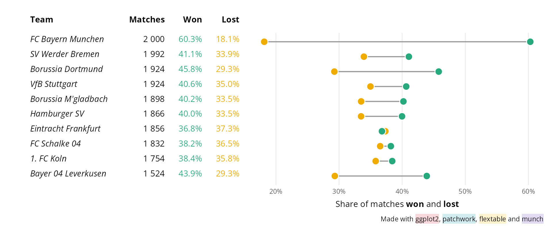
The rows of the table are aligned with the categories of the plot (see 15).
6.1 Markdown in cells
as_paragraph_md() turns markdown into a flextable paragraph. It is used
in mk_par() as as_paragraph(), and it is vectorised: each element gives
the paragraph of a row, so a column of markdown is formatted in one call.
dat <- data.frame(
  property = c("Speed", "Weight", "Status"),
  value = c("**120** km/h", "*1.2* t", "~~draft~~ `final`")
)

flextable(dat) |>
  mk_par(
    j = "value",
    value = as_paragraph_md(value, font_family_mono = "Liberation Mono")
  ) |>
  autofit()
property |
value |
|---|---|
Speed |
120 km/h |
Weight |
1.2 t |
Status |
draft final |
It works the same way in the header, or in a footer:
flextable(head(iris, 3)) |>
  mk_par(
    j = 1:4, part = "header",
    value = as_paragraph_md(c(
      "*Sepal* **Length**", "*Sepal* **Width**",
      "*Petal* **Length**", "*Petal* **Width**"
    ))
  ) |>
  autofit()
Sepal Length |
Sepal Width |
Petal Length |
Petal Width |
Species |
|---|---|---|---|---|
5.1 |
3.5 |
1.4 |
0.2 |
setosa |
4.9 |
3.0 |
1.4 |
0.2 |
setosa |
4.7 |
3.2 |
1.3 |
0.2 |
setosa |
6.1.1 What markdown can contain
The table below shows each syntax supported, written on the left and rendered on the right.
syntax <- data.frame(
feature = c(
"Bold and italic", "Code", "Strikethrough",
"Superscript and subscript", "Image", "Equation"
),
markdown = c(
"**bold**, *italic*, ***both***",
"`mk_par()`",
"~~removed~~",
"m^2^, H~2~O",
"",
"$\\bar{x} = \\frac{1}{n}\\sum_{i=1}^{n} x_i$"
)
)
syntax$rendered <- syntax$markdown
flextable(syntax) |>
mk_par(j = "markdown", value = as_paragraph(as_chunk(markdown,
props = fp_text_default(font.family = "Inconsolata")))) |>
mk_par(
j = "rendered",
value = as_paragraph_md(rendered, font_family_mono = "Liberation Mono")
) |>
set_header_labels(feature = "Feature", markdown = "Markdown",
rendered = "Rendered") |>
valign(valign = "center", part = "body") |>
autofit()Feature |
Markdown |
Rendered |
|---|---|---|
Bold and italic |
**bold**, *italic*, ***both*** |
bold, italic, both |
Code |
`mk_par()` |
mk_par() |
Strikethrough |
~~removed~~ |
removed |
Superscript and subscript |
m^2^, H~2~O |
m2, H2O |
Image |
 |
|
Equation |
$\bar{x} = \frac{1}{n}\sum_{i=1}^{n} x_i$ |
|

Equations need the package ‘equatags’; they are flextable equations (see
as_equation()), with the size and the color of the text around them.
Each element is a single paragraph: titles, lists and code blocks are not supported.
6.2 The same table in every format
The paragraphs made by as_paragraph_md() are ordinary flextable
paragraphs. The markdown is read once, in R, and the table is then
rendered by flextable as any other: in Word, PowerPoint, HTML, PDF, RTF,
Typst, and as an image.
The table of syntaxes above, in a Word document. Inline code is written
with the font “Liberation Mono” (argument font_family_mono), registered
by ‘gdtools’ and embedded in the document with
officer::docx_embed_font(), so that it displays the same on any machine
(see 10.6.1):
library(officer)
gdtools::register_liberationmono()
# [1] TRUE
ft_syntax <- flextable(syntax[, c("feature", "rendered")]) |>
  mk_par(
    j = "rendered",
    value = as_paragraph_md(rendered, font_family_mono = "Liberation Mono")
  ) |>
  set_header_labels(feature = "Feature", rendered = "Rendered") |>
  valign(valign = "center", part = "body") |>
  autofit()

doc <- read_docx() |>
  docx_embed_font(font_family = "Liberation Mono") |>
  body_add_flextable(ft_syntax)
print(doc, target = "reports/munch_markdown_word.docx")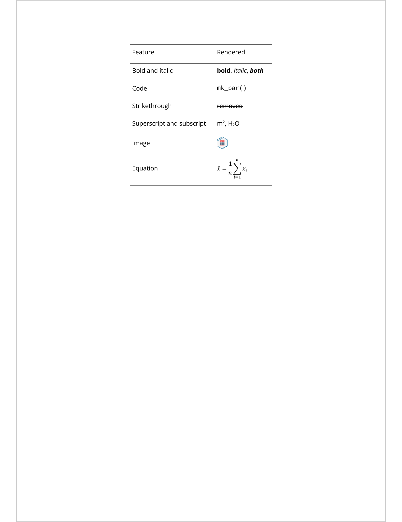
And in a PowerPoint presentation, without the image, as PowerPoint does not support images in tables (see 5.6). Fonts can not be embedded in a presentation with officer: a reader who does not have “Liberation Mono” sees a replacement font.
ft_syntax_ppt <- ft_syntax |>
  delete_rows(i = ~ feature == "Image", part = "body")

save_as_pptx(ft_syntax_ppt, path = "reports/munch_markdown_powerpoint.pptx")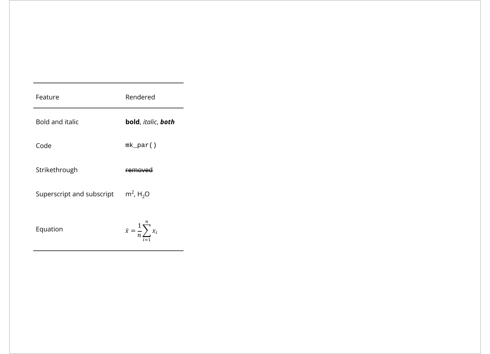
The same goes for save_as_rtf(), save_as_html() and save_as_image().
This is the difference with as_qmd() (see 8.4), which
delegates the markdown to Quarto and therefore only works in Quarto
documents, but supports cross-references and the whole Quarto markdown.
6.3 One paragraph, in a table and in a plot
Markdown does not cover everything: colors, highlighting or font sizes
need flextable chunks (colorize(), as_highlight(), as_chunk() with
fp_text_default()…). A paragraph built with as_paragraph() can be
used in a cell with mk_par(), and in a ‘ggplot2’ theme with
element_chunks(): it is written once, and rendered the same way in both.
note <- as_paragraph(
  as_b("Note: "), "values in ",
  colorize("orange", color = "#EFAC00"), " are ",
  as_highlight("provisional", color = "#FFF3CD"), "."
)

ft <- flextable(head(mtcars[, 1:4], 3)) |>
  add_footer_lines(values = note) |>
  autofit()
ft
mpg |
cyl |
disp |
hp |
|---|---|---|---|
21.0 |
6 |
160 |
110 |
21.0 |
6 |
160 |
110 |
22.8 |
4 |
108 |
93 |
Note: values in orange are provisional. | |||
ggplot(mtcars, aes(wt, mpg)) +
  geom_point() +
  labs(caption = "x") +
  theme_minimal(base_family = "Open Sans") +
  theme(plot.caption = element_chunks(note))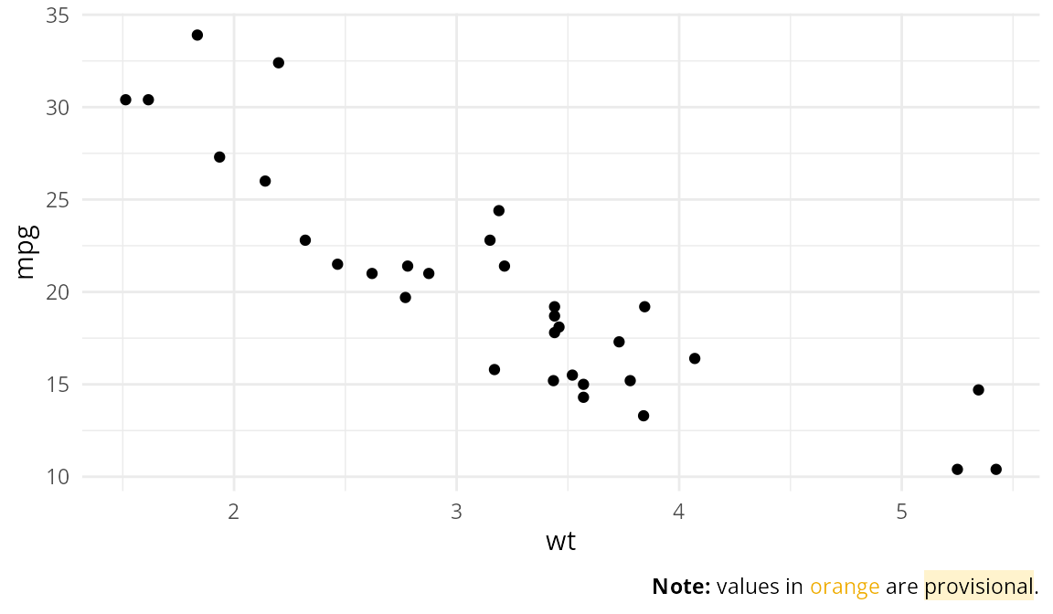
6.4 And in ggplot2
In ‘ggplot2’, element_md() replaces element_text() to write markdown in
titles, axis titles, axis labels, legends and facet strips;
element_chunks() takes a flextable paragraph; geom_text_md() and
geom_label_md() write markdown in the panel.
ggplot(penguins, aes(bill_length_mm, flipper_length_mm)) +
  geom_point(aes(colour = species), size = 2, alpha = .8) +
  geom_label_md(
    label = "**Gentoo** have *longer* flippers",
    x = 32, y = 230, fill = "white", hjust = 0
  ) +
  labs(
    title = "Flipper and bill **length** *(millimeters)*",
    x = "Bill length *(mm)*", y = "Flipper length *(mm)*",
    colour = "*Species*"
  ) +
  theme_minimal(base_family = "Open Sans") +
  theme(
    plot.title = element_md(),
    axis.title = element_md(),
    legend.title = element_md()
  )
# Warning: Removed 2 rows containing missing values or values outside the scale range
# (`geom_point()`).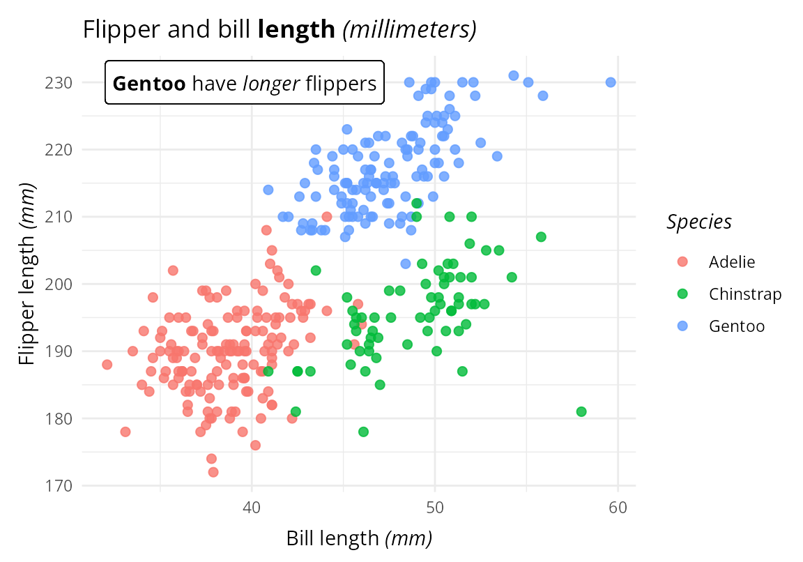
The articles of ‘munch’ cover the details:
6.5 Good to know
- One paragraph per element. Markdown titles, lists and code blocks are not supported; for multi-block markdown in plots, see the package ‘marquee’.
-
Plots and images need a compatible graphic device. Text is measured
with ‘systemfonts’, so plots are drawn correctly by the devices that use
it: ‘ragg’, ‘svglite’ and ‘ggiraph’. With knitr, set
knitr::opts_chunk$set(dev = "ragg_png"); in RStudio, choose ‘AGG’ as graphics backend. Tables rendered in Word, PowerPoint, HTML, PDF or RTF are not concerned. - Fonts must be available. As for any flextable rendered as an image, use a font installed on the machine or registered with ‘gdtools’ (see 10).