Chapter 4 officer for Word

4.1 Add contents

To add paragraphs of text, tables, images to a Word document, you have to use one of the body_add_* functions:

• body_add_blocks()
• body_add_break()
• body_add_caption()
• body_add_docx()
• body_add_fpar()
• body_add_gg()
• body_add_img()
• body_add_list()
• body_add_par()
• body_add_plot()
• body_add_table()
• body_add_toc()

They all have the same output and the same first argument: the R object representing the Word document, these functions are all taking as first input the document that needs to be filled with some R content and are all returning the document, that has been augmented with the new R content(s) after the function call.

x <- body_add_par(x, "Level 1 title", style = "heading 1")

These functions are all creating one or more top level elements, either paragraphs, either tables.

4.1.1 Tables

The tabular reporting topic is handled by ‘officer’ using the body_add_table() function. The function is rendering data.frame as Word tables with few formatting options available; it is recommended to use the ‘flextable’ package for more advanced formatting needs.

The body_add_table() function adds a data.frame as a Word table whose formatting is defined in the document template, a group of settings that can be applied to a table. The settings include formatting for the overall table, rows, columns, etc.

You can activate the “conditional formatting” instructions, i.e. a style for the first or last row, the first or last column and a style for the row or column strips.

• first_row: apply or remove formatting from the first row in the table.
• first_column: apply or remove formatting from the first column in the table.
• last_row: apply or remove formatting from the last row in the table.
• last_column: apply or remove formatting from the last column in the table.
• no_hband: don’t display odd and even rows.
• no_vband: don’t display odd and even columns.

dat <- cbind(data.frame(cars = row.names(mtcars)),
             mtcars)
head(dat)

cars	mpg	cyl	disp	hp	drat	wt	qsec	vs	am	gear	carb
character	numeric	numeric	numeric	numeric	numeric	numeric	numeric	numeric	numeric	numeric	numeric
Mazda RX4	21.0	6	160	110	3.9	2.6	16.5	0	1	4	4
Mazda RX4 Wag	21.0	6	160	110	3.9	2.9	17.0	0	1	4	4
Datsun 710	22.8	4	108	93	3.9	2.3	18.6	1	1	4	1
Hornet 4 Drive	21.4	6	258	110	3.1	3.2	19.4	1	0	3	1
Hornet Sportabout	18.7	8	360	175	3.1	3.4	17.0	0	0	3	2
Valiant	18.1	6	225	105	2.8	3.5	20.2	1	0	3	1
n: 6

doc_table <- read_docx(path = "templates/template_demo.docx") |>
  body_add_table(head(dat, n = 20), style = "Table") |> 
  body_add_break() |> 
  body_add_table(head(dat, n = 20), style = "Table", 
                 first_column = TRUE)

print(doc_table, target = "static/office/example_table.docx")

static/office/example_table.docx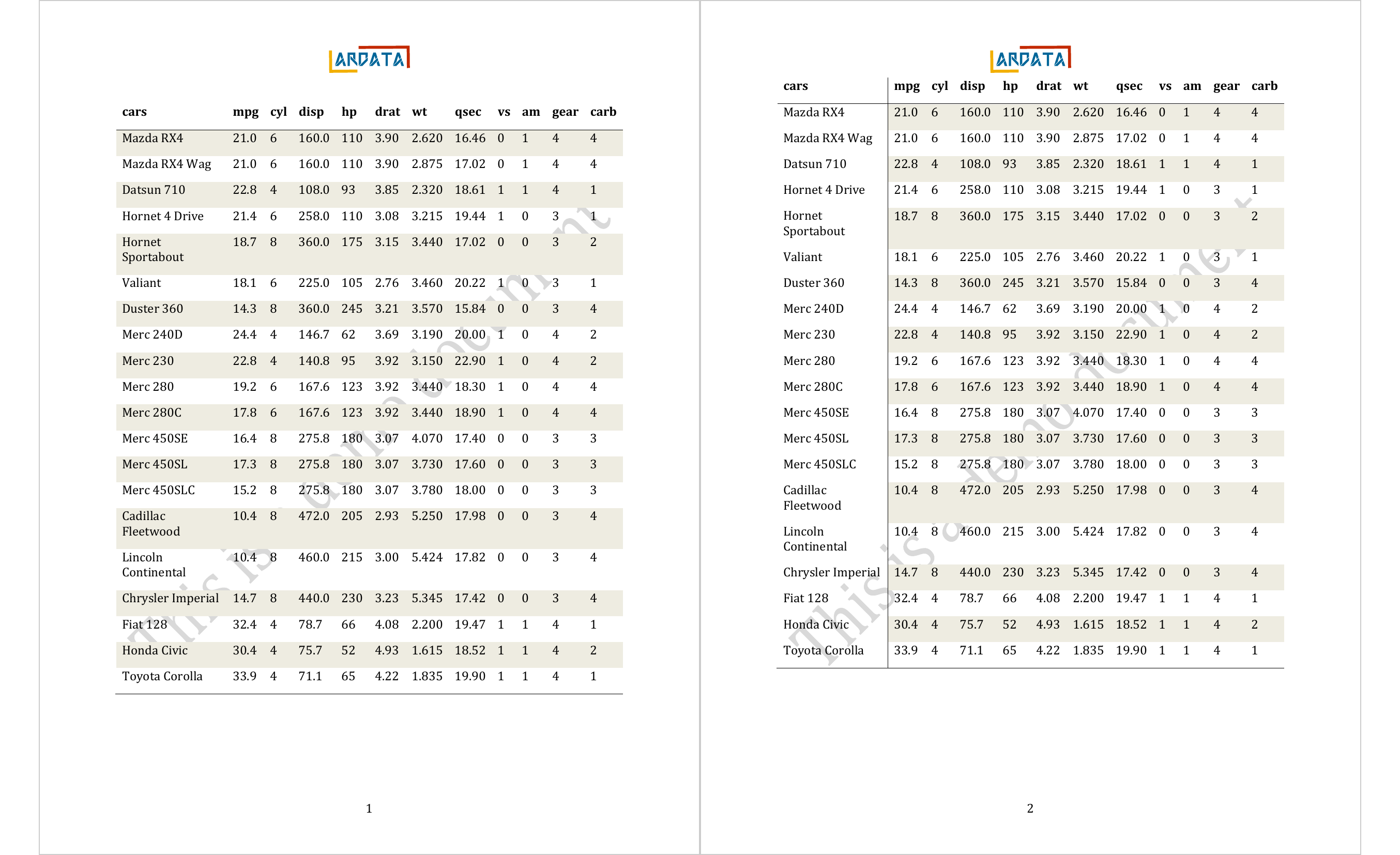

4.1.2 Paragraphs

The package makes it very easy to use paragraph styles. You can incrementally add a text associated with a paragraph style.

The function is not vectorized, it is planned to implement this vectorization in the future.

To add a text paragraph, use the body_add_paragraph() function. The function requires 3 arguments, the target document, the text to be used in the new paragraph, and the paragraph style to be used.

read_docx() |> 
  body_add_par(value = "Hello World!", style = "Normal") |> 
  body_add_par(value = "Salut Bretons!", style = "centered") |> 
  print(target = "static/office/example_par.docx")

static/office/example_par.docx

4.1.3 Titles

A title is a paragraph. To add a title, use body_add_par() with the style argument set to the corresponding title style.

read_docx() |> 
  body_add_par(value = "This is a title 1", style = "heading 1") |> 
  body_add_par(value = "This is a title 2", style = "heading 2") |> 
  body_add_par(value = "This is a title 3", style = "heading 3") |> 
  print(target = "static/office/example_titles.docx")

static/office/example_titles.docx

4.1.4 Lists

Bulleted and numbered lists are created in two steps: build list items with list_item(), assemble them into a block_list_items(), and insert the result with body_add_list(). Each item carries an integer level (starting at 1) that controls nesting; list_type selects "bullet" (unordered) or "decimal" (numbered).

items <- block_list_items(
  list_item("First top-level item",                       level = 1),
  list_item("A nested item",                              level = 2),
  list_item("Another nested item",                        level = 2),
  list_item("Back to top level",                          level = 1),
  list_type = "bullet"
)

read_docx() |>
  body_add_par("Bulleted list", style = "heading 2") |>
  body_add_list(items) |>
  print(target = "static/office/example_bullet_list.docx")

static/office/example_bullet_list.docx

A list_item() accepts either a plain string (converted to an fpar() internally) or a full fpar(). The second form lets you mix formatting inside an item — bold, colour, hyperlinks, etc. — while keeping the list structure:

items <- block_list_items(
  list_item(fpar(
    ftext("Install", fp_text_lite(bold = TRUE)),
    " the package"
  ), level = 1),
  list_item("Load it with library()",                     level = 1),
  list_item(fpar(
    "Read the ",
    ftext("documentation", fp_text_lite(italic = TRUE))
  ), level = 1),
  list_type = "decimal"
)

read_docx() |>
  body_add_par("Numbered list", style = "heading 2") |>
  body_add_list(items) |>
  print(target = "static/office/example_numbered_list.docx")

static/office/example_numbered_list.docx

The same block_list_items object can be inserted into a PowerPoint slide via ph_with() — see the Lists section of the PowerPoint chapter.

4.1.5 Tables of contents

A TOC (Table of Contents) is a Word computed field, table of contents is built by Word. The TOC field will collect entries using heading styles or another specified style.

Note: you have to update the fields with Word application to reflect the correct page numbers. See update the fields

Use function body_add_toc() to insert a TOC inside a Word document.

doc_toc <- read_docx(path = "templates/word_example.docx") |>
  body_add_par("Table of Contents", style = "heading 1") |> 
  body_add_toc(level = 2) |> 
  body_add_par("Table of figures", style = "heading 1") |> 
  body_add_toc(style = "Image Caption") |> 
  body_add_par("Table of tables", style = "heading 1") |> 
  body_add_toc(style = "Table Caption")

print(doc_toc, target = "static/office/example_toc.docx")

static/office/example_toc.docx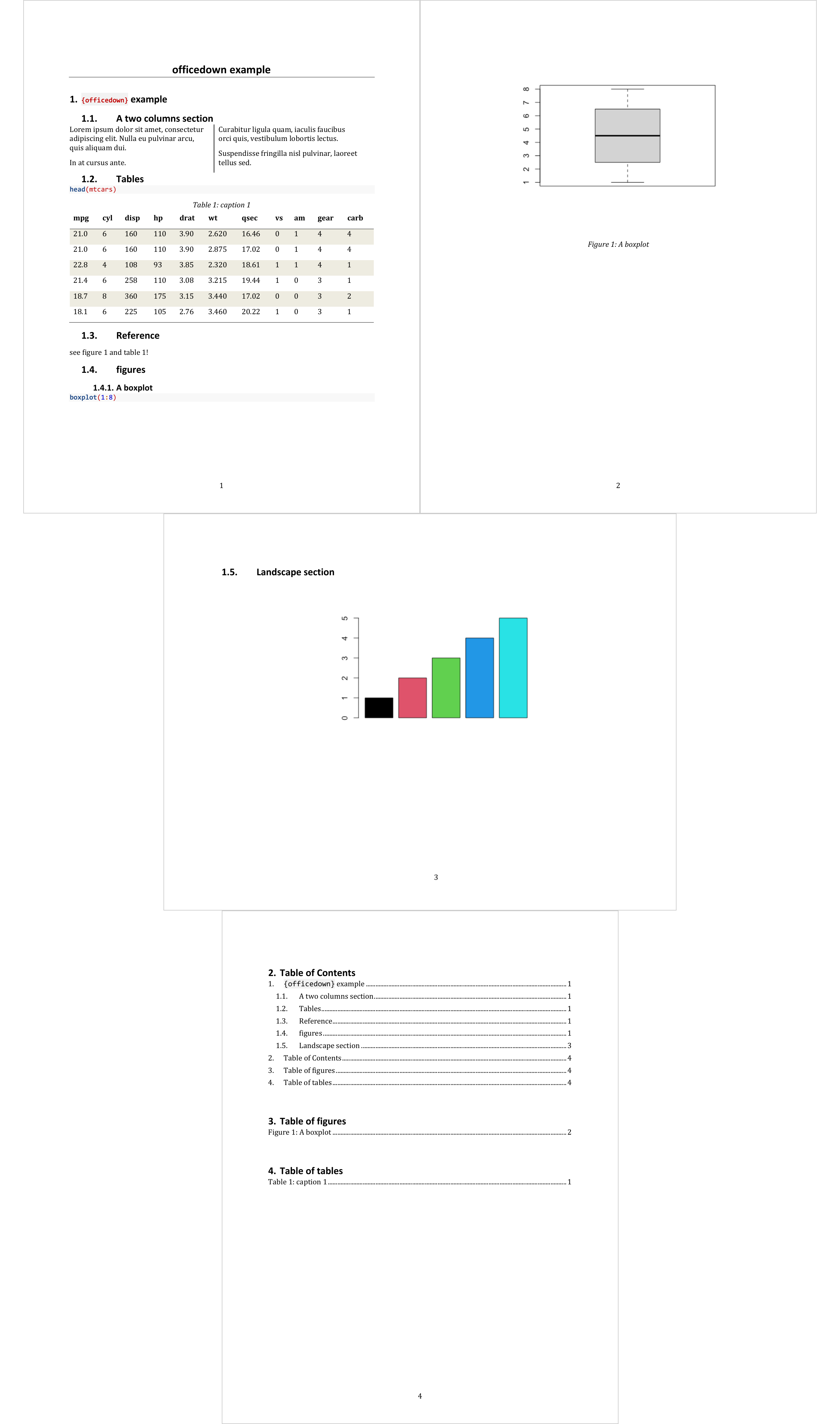

4.1.6 Images

Images are specific because they are part of a paragraph. This means you can mix text and images in a paragraph. An image is always rendered in a paragraph. Functions body_add_img() is a sugar function that wrap an image into a paragraph. It accepts various image formats: png, jpeg or emf.

img.file <- file.path( R.home("doc"), "html", "logo.jpg" )

read_docx() |>
  body_add_img(src = img.file, height = 1.06, width = 1.39, style = "centered") |>
  print(target = "static/office/example_image.docx")

static/office/example_image.docx

4.1.7 Floating images

By default, images added with body_add_img() or external_img() are inline: the image occupies a rectangular area in the line of text and the paragraph flows around it like a word. A floating image is anchored at a position on the page (relative to the margin, the page or the column), and the surrounding text wraps around it — the same behaviour as “In Front of Text / Square / Tight” wrap options in Word’s image panel.

floating_external_img() creates a run that embeds a floating image. It is used inside fpar() alongside regular text runs:

img.file <- file.path(R.home("doc"), "html", "logo.jpg")

floatimg <- floating_external_img(
  src = img.file, width = 0.7, height = 0.53,
  pos_x = 0, pos_y = 0,
  pos_h_from = "margin", pos_v_from = "margin",
  wrap_type = "square"
)

long_text <- paste(rep("Some text that wraps around the logo.", 20),
                   collapse = " ")

read_docx() |>
  body_add_fpar(fpar(floatimg, long_text)) |>
  print(target = "static/office/example_floating_img.docx")

static/office/example_floating_img.docx

Key arguments:

• pos_x, pos_y — offset of the image anchor (in inches by default, see unit).
• pos_h_from, pos_v_from — reference frame for the offset: "margin" (default), "page", "column" (horizontal) or "paragraph" (vertical).
• wrap_type — how surrounding text flows around the image: "square" (default), "tight", "through", "topAndBottom" or "none".
• wrap_dist_* — margins between the image and the wrapped text.

4.1.8 Plots from ‘ggplot2’

Function body_add_gg() is also a sugar function that wrap an image generated from a ggplot into a paragraph.

library(ggplot2)

gg <- ggplot(data = iris, aes(Sepal.Length, Petal.Length)) + 
  geom_point()

doc_gg <- read_docx()
doc_gg <- body_add_gg(x = doc_gg, value = gg, style = "centered")

The size of the Word document can be used to maximize the size of the graphic to be produced.

word_size <- docx_dim(doc_gg)
word_size

# $page
#     width    height 
#  8.263889 11.694444 
# 
# $landscape
# [1] FALSE
# 
# $margins
#       top    bottom      left     right    header    footer 
# 0.9840278 0.9840278 0.9840278 0.9840278 0.4916667 0.4916667

width <- word_size$page['width'] - word_size$margins['left'] - word_size$margins['right']
height <- word_size$page['height'] - word_size$margins['top'] - word_size$margins['bottom']

doc_gg <- body_add_gg(x = doc_gg, value = gg, 
                      width = width, height = height, 
                      style = "centered")

print(doc_gg, target = "static/office/example_gg.docx")

static/office/example_gg.docx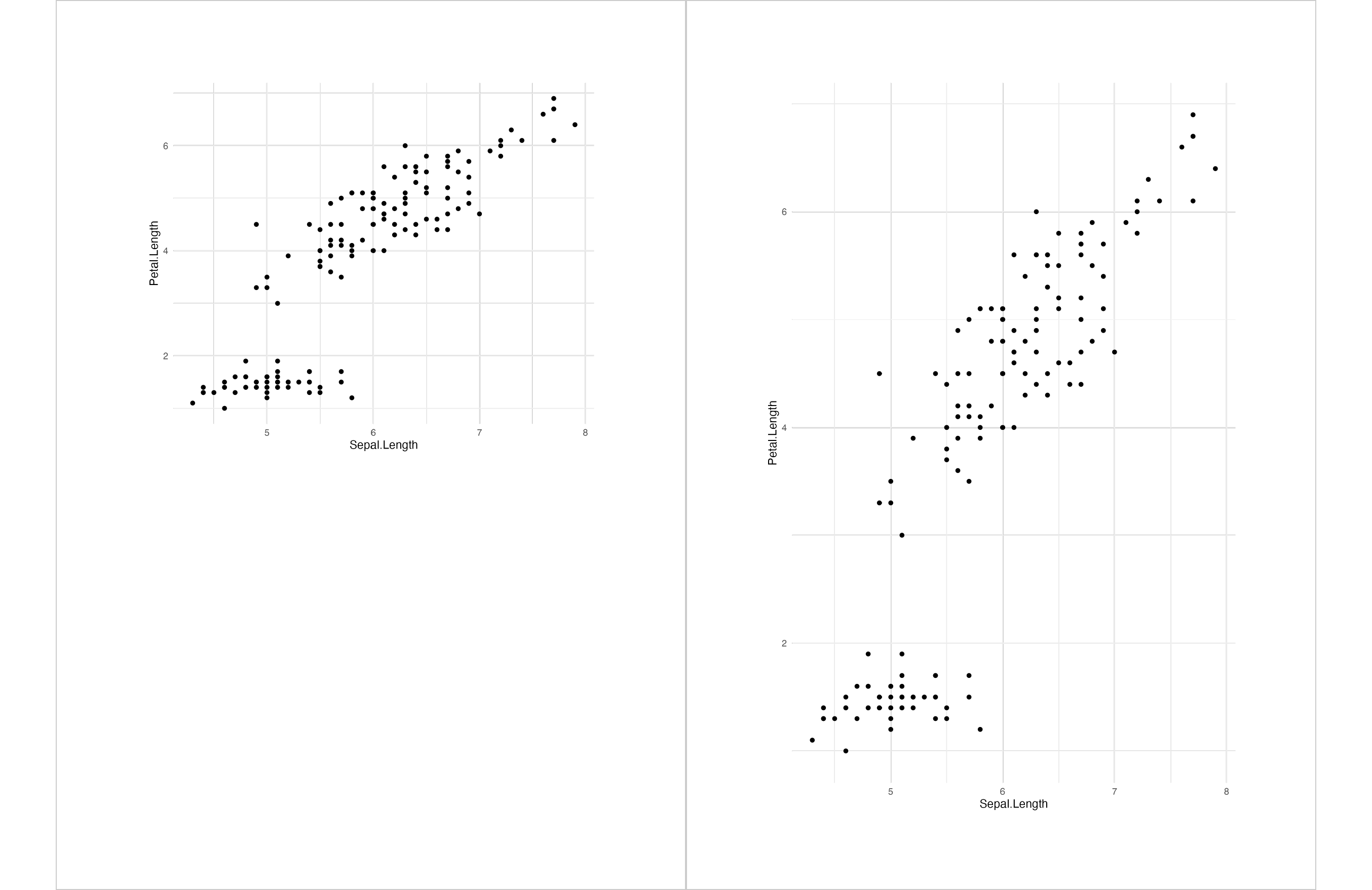

4.1.9 Base plot

To add a standard R graphic, use the body_add_plot function with plot_instr which contains the graphic instructions to be executed to produce a single graphic.

doc <- read_docx()
doc <- body_add_plot(doc,
    width = width, height = height,
    value = plot_instr(
      code = {barplot(1:5, col = 2:6)}),
      style = "centered")
print(doc, target = "static/office/example_word_plot_instr.docx")

static/office/example_word_plot_instr.docx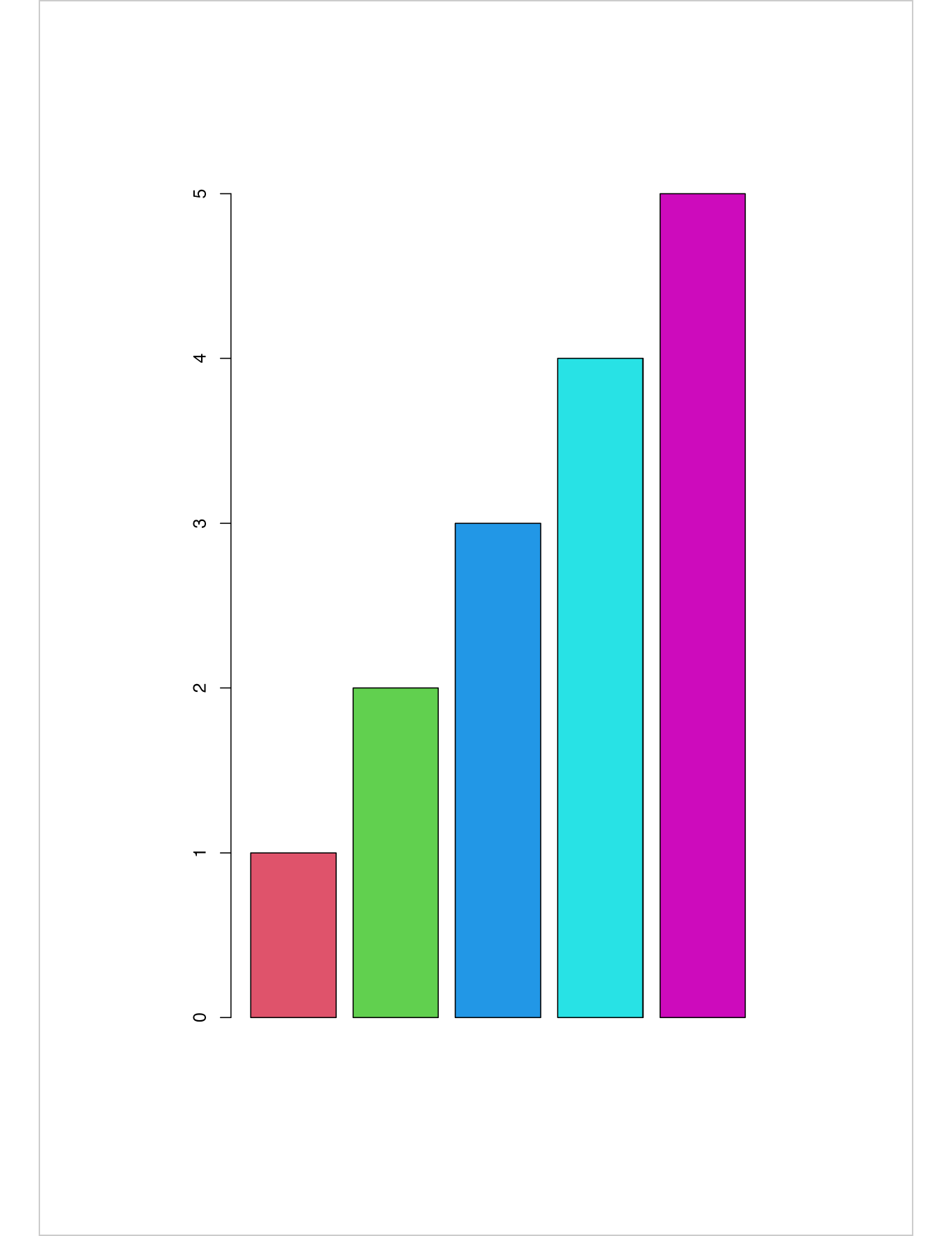

4.1.10 Microsoft charts

The ‘mschart’ package allows you to create native office graphics that can be used with ‘officer’. The body_add_chart function must be used to generate an office chart in Word.

library(mschart)

my_barchart <- ms_barchart(data = browser_data,
  x = "browser", y = "value", group = "serie")
my_barchart <- chart_settings( x = my_barchart,
  dir="vertical", grouping="clustered", gap_width = 50 )

read_docx() |> 
  body_add_chart(chart = my_barchart, style = "centered") |> 
  print(target = "static/office/example_word_chart.docx")

static/office/example_word_chart.docx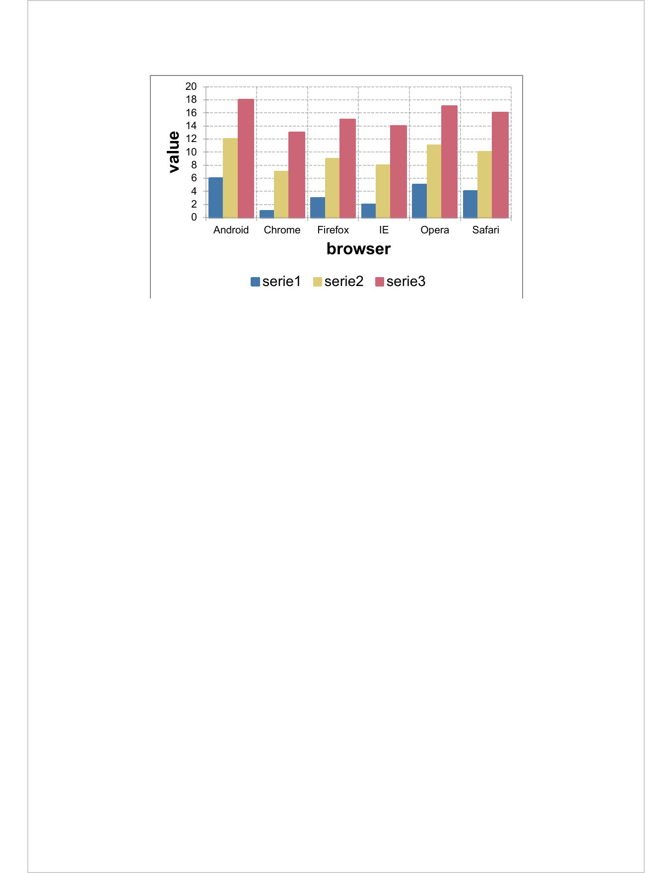

4.1.11 Page breaks

Page breaks are handy for formatting a Word document. They allow you to control where your document should move to the next page, such as at the end of a chapter or section.

Use function body_add_break() to add a page break in the Word document.

library(ggplot2)
library(flextable)

gg <- ggplot(data = iris, aes(Sepal.Length, Petal.Length)) + 
  geom_point()

ft <- flextable(head(iris, n = 10))
ft <- set_table_properties(ft, layout = "autofit")

read_docx() |> 
  body_add_par(value = "dataset iris", style = "heading 2") |> 
  body_add_flextable(value = ft ) |> 
  
  body_add_break() |> 

  body_add_par(value = "plot examples", style = "heading 2") |> 
  body_add_gg(value = gg, style = "centered") |> 
  
  print(target = "static/office/example_break.docx")

static/office/example_break.docx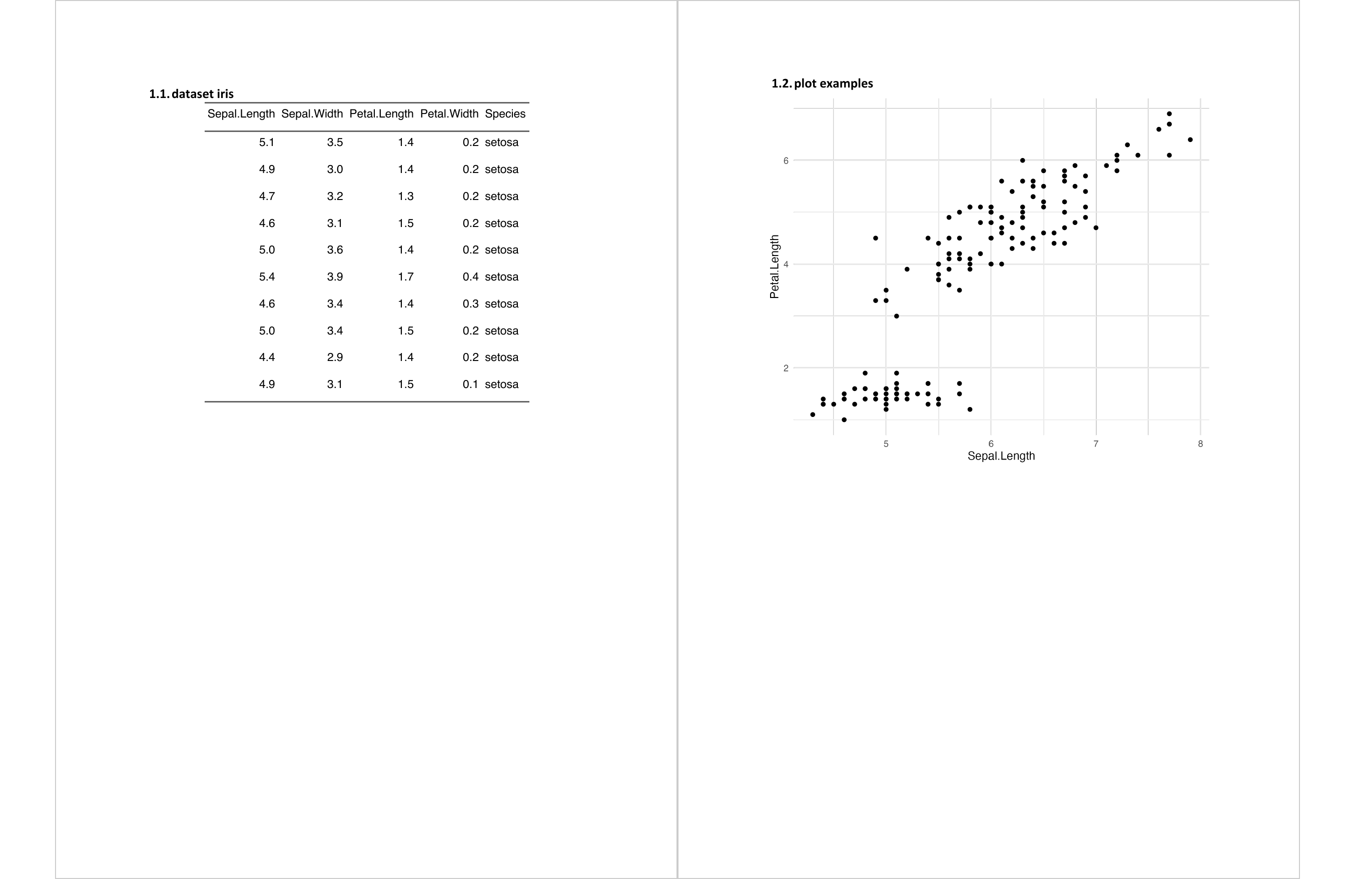

4.1.12 External documents

Integrating a previously-created Word document into another document is useful when certain parts of a report are written manually but assembled programmatically into a final deliverable. The document to be inserted must be in docx format.

Two functions are available, with different trade-offs:

• body_add_docx(src) inserts the source document as an external altChunk. The target file keeps a reference to the source fragment; Word actually imports it when the document is opened. The source’s styles are preserved as they are, late-bound at open time.
• body_import_docx(src, ...) reads the source at print() time and merges its body and footnotes into the target. Styles are not copied across: unknown styles must be remapped to target-document styles via the par_style_mapping, run_style_mapping and tbl_style_mapping arguments, otherwise a warning is emitted and the default styles are used. Numberings from the source are copied over.

Use body_add_docx() when you want loose, fast assembly of independent documents. Use body_import_docx() when you want a truly homogeneous final document with a single style set, typically for template-based reports.

4.1.12.1 Embedding with body_add_docx()

read_docx() |>
  body_add_par(value = "An external document", style = "heading 1") |>
  body_add_docx(src = "static/office/example_break.docx") |>
  print(target = "static/office/example_add_docx.docx")

static/office/example_add_docx.docx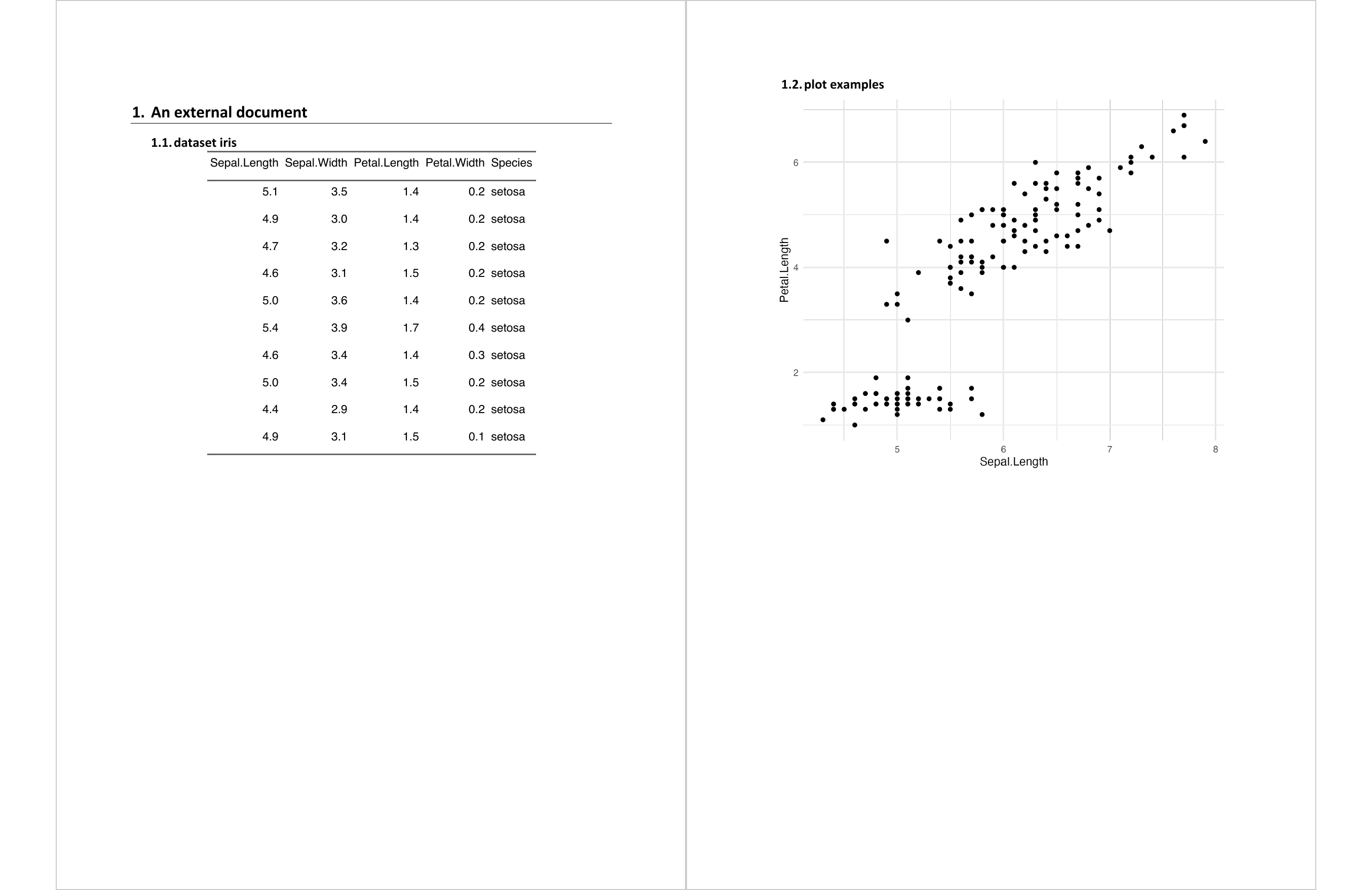

This can be advantageous when you are generating huge documents and the generation is getting slower and slower.

It is necessary to generate smaller documents and to design a main script that inserts the different documents into a main Word document. The following script illustrates the strategy:

library(uuid)

ft <- flextable(iris)
ft <- set_table_properties(ft, layout = "autofit")

gg_plot <- ggplot(data = iris ) +
  geom_point(mapping = aes(Sepal.Length, Petal.Length))

tmpdir <- tempfile()
dir.create(tmpdir, showWarnings = FALSE, recursive = TRUE)
tempfiles <- file.path(tmpdir, paste0(UUIDgenerate(n = 10), ".docx") )

for(i in seq_along(tempfiles)) {
  doc <- read_docx()
  doc <- body_add_par(doc, value = "", style = "Normal")
  doc <- body_add_gg(doc, value = gg_plot, style = "centered")
  doc <- body_add_par(doc, value = "", style = "Normal")
  doc <- body_add_flextable(doc, value = ft)
  temp_file <- tempfile(fileext = ".docx")
  print(doc, target = tempfiles[i])
}

# tempfiles contains all generated docx paths

main_doc <- read_docx()
for(tempfile in tempfiles){
  main_doc <- body_add_docx(main_doc, src = tempfile)
}
print(main_doc, target = "static/office/example_huge.docx")

4.1.12.2 Importing with body_import_docx()

body_import_docx() reads the source and merges its body and footnotes into the target document. Because styles are not carried over, any style used in the source that does not exist in the target must be remapped explicitly.

The chunk below prepares a source document with a custom paragraph style MyNote (hidden from the output). The import step then remaps MyNote to the standard Normal style of the target document:

read_docx() |>
  body_add_par("A merged document", style = "heading 1") |>
  body_import_docx(
    src = "static/office/example_import_source.docx",
    par_style_mapping = list(Normal = "MyNote")
  ) |>
  print(target = "static/office/example_import_docx.docx")

static/office/example_import_docx.docx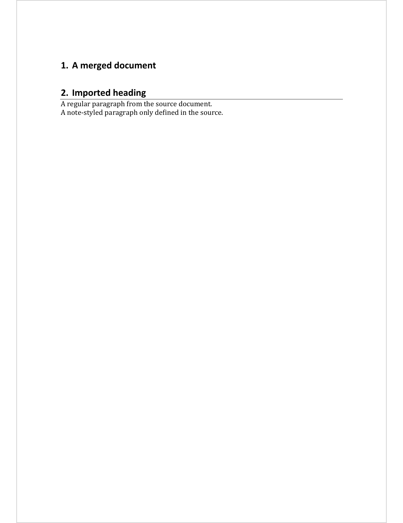

par_style_mapping = list(Normal = "MyNote") reads as: in the source, any paragraph styled MyNote should be re-tagged Normal in the target. The same shape applies to run_style_mapping (character styles) and tbl_style_mapping (table styles). Styles that already exist in the target need no mapping.

4.2 Add Sections

A section affects preceding paragraphs or tables (see Word Sections).

Usually, starting with a continous section and ending with the section you defined is enough.

To format your content in a section, you should use the body_end_block_section function. First you need to define the section with the block_section function, which takes an object returned by the prop_section function. It is prop_section() that allows you to define the properties of your section.

Let’s first create a document and add a graphic:

library(ggplot2)

gg <- ggplot(data = iris, aes(Sepal.Length, Petal.Length)) + 
  geom_point()

doc_section_1 <- read_docx()
doc_section_1 <- body_add_gg(
  x = doc_section_1, value = gg, 
  width = 9, height = 6,
  style = "centered")

Now, let’s add a section that will set the previously graphic display in a landscape oriented page.

ps <- prop_section(
  page_size = page_size(orient = "landscape"),
  type = "oddPage")

doc_section_1 <- body_end_block_section(
  x = doc_section_1, 
  value = block_section(property = ps))

That’s it, let’s add the graphic again to see it display at the end of the document in the default section:

doc_section_1 <- body_add_gg(
  x = doc_section_1, value = gg,
  width = 6.29, height = 9.72,
  style = "centered"
)

print(doc_section_1, target = "static/office/example_landscape_gg.docx")

static/office/example_landscape_gg.docx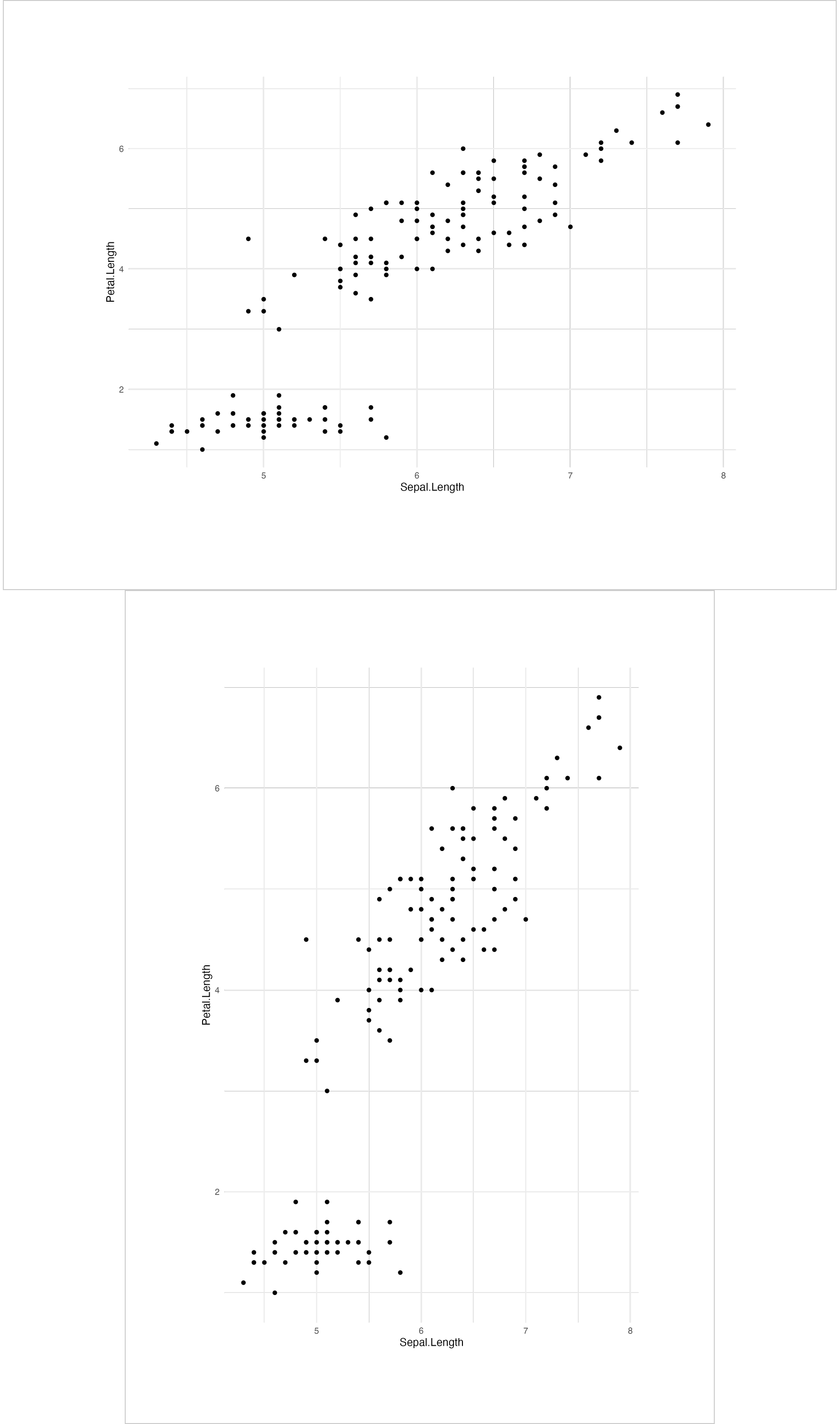

4.2.1 Supported features

Most of the properties of Word sections are available with the ‘officer’ package: page size, page margins, section type (oddPage, continuous, nextColumn) and columns. The ability to link a header or footer to a section is not (yet) implemented.

Section properties are defined with function prop_section with arguments:

• page_size: page dimensions defined with function page_size().
• page_margins: page margins defined with function page_margins().
• type : section type (“continuous”, “evenPage”, “oddPage”, …).
• section_columns: section columns defined with function section_columns().

4.2.2 How to manage sections

The body_end_block_section function is usually used twice. The first time to close the previous section (and thus start the new one) and then another section to close the second one. All content between the end of the first section and the end of the second section will be arranged according to the rules defined for the second section.

Let’s illustrate the principle with a graphic that need to be in a landscape oriented page.

1. A paragraph is added.
2. We add an end of section (we use a continuous section for this) to let the first paragraph fit in the default section.
3. Add the graphic.
4. We add an end of section that will apply to the graphic (we reuse the property that allows to have a section oriented in landscape).

doc_section_2 <- read_docx() |> 
  body_add_par("This is a dummy text. It is in a continuous section") |> 
  body_end_block_section(block_section(prop_section(type = "continuous"))) |> 
  body_add_gg(value = gg, width = 7, height = 5, style = "centered") |> 
  body_end_block_section(block_section(property = ps))

print(doc_section_2, target = "static/office/example_landscape_gg2.docx")

static/office/example_landscape_gg2.docx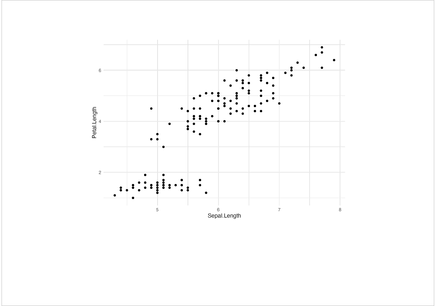

Note that if you add a section break at the end of the document with a different orientation than the default, it generates a last page that is empty. This is a behavior of Word and there is only one solution: using a template where the default orientation is the same as the last section break. For example, a default landscape orientation if you insert a landscape oriented section at the end of the document.

Now, let’s illustrate a complex layout. We are going to add two sections oriented in landscape. The first will contain a table, the second will contain long text separated into two columns. The final result will be a landscape oriented page containing a table and then text spread over two columns (and of course this famous extra blank page).

landscape_one_column <- block_section(
  prop_section(
    page_size = page_size(orient = "landscape"), type = "continuous"
  )
)
landscape_two_columns <- block_section(
  prop_section(
    page_size = page_size(orient = "landscape"), type = "continuous",
    section_columns = section_columns(widths = c(4, 4))
  )
)

doc_section_3 <- read_docx() |>
  body_add_table(value = head(mtcars), style = "table_template") |>
  body_end_block_section(value = landscape_one_column) |> 
  body_add_par(value = paste(rep(letters, 60), collapse = " ")) |>
  body_end_block_section(value = landscape_two_columns)

print(doc_section_3, target = "static/office/example_complex_section.docx")

static/office/example_complex_section.docx

4.2.3 Sugar functions

In addition to the generic function body_end_block_section, some utility functions are available to be used as shortcuts:

• body_end_section_landscape()
• body_end_section_portrait()
• body_end_section_columns()
• body_end_section_columns_landscape()
• body_end_section_continuous()

4.3 Remove content

The function body_remove() lets you remove content from a Word document. This function is often to be used with a cursor_* function.

For illustration purposes, we will reuse document produced here as initial document and the last three paragraphs will be removed.

my_doc <- read_docx(path = "static/office/example_break.docx")

my_doc <- body_remove(my_doc) |> cursor_end()
my_doc <- body_remove(my_doc) |> cursor_end()
my_doc <- body_remove(my_doc) |> cursor_end()

print(my_doc, target = "static/office/example_remove.docx")

static/office/example_remove.docx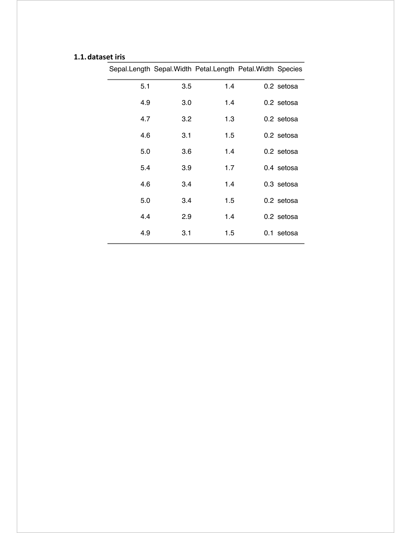

4.4 Content Replacement

When it comes to replacing content in an existing Word document, there is no straightforward solution using only the ‘officer’ package. This is due to the limitations of Microsoft Word’s design as a manual editing program with limited automation capabilities. There are a few reasons why content replacement can be challenging:

• Word does not provide a consistent built-in mechanism for marking a specific target area in a document, making it difficult to identify and replace specific content.
• Word arranges typed words into “run” chunks, each containing identically formatted text. However, Word’s handling of run chunks can be inconsistent, especially when there are pauses in typing. For example, typing “he” and then “llo” may result in two separate runs for “he” and “llo,” making it harder to detect and replace the complete word “hello” programmatically.

While the ‘officer’ package does offer some functions for content replacement, it is important to note their limitations and potential difficulties in usage. The approach chosen by ‘officer’ involves using bookmarks placed inside paragraphs, which presents its own challenges:

• Placing bookmarks on successive paragraphs renders them unusable.
• Placing bookmarks on single words within a paragraph allows for their use.

The existing ‘officer’ functions for content replacement replace entire paragraphs where the bookmark is located. Unfortunately, they do not allow for partial text replacement within a paragraph, and the replaced paragraph no longer retains the original bookmark.

To preserve bookmarks after replacing the containing paragraph, you need to re-inject the bookmarks using the run_bookmark() function.

The ‘officer’ package provides the following functions for content replacement, but we do not recommend using them due to their limitations (we will deprecate these functions in the future):

• body_replace_all_text()
• headers_replace_all_text()
• footers_replace_all_text()
• body_replace_text_at_bkm()
• body_replace_img_at_bkm()
• headers_replace_text_at_bkm()
• headers_replace_img_at_bkm()
• footers_replace_text_at_bkm()
• footers_replace_img_at_bkm()

Instead, we recommend using the ‘doconv’ package, which offers more flexibility and advanced features for manipulating Word documents. ‘doconv’ allows you to perform complex tasks such as updating calculated fields, including tables of contents and document property references.

With ‘doconv’, you can replace specific chunks of text rather than whole paragraphs. You can find detailed instructions on how to perform content replacement and utilize other features of ‘doconv’ in the article https://www.ardata.fr/en/post/2022/08/25/doconv-0-1-4-is-out/.

To enable text replacement without using body_replace_* functions, ‘officer’ provides functions for simple text replacement without bookmark management:

• the officer::run_word_field() function, which allows calculated field insertions. Note it’s probably easier to set them manually.
• the set_doc_properties() function, which adds values to be replaced in the document (thanks to calculated fields), and that can be updated with doconv::docx_update().

The following example shows a template with Word computed fields, how to replace the values and update the document with doconv::docx_update().

a word template with computed fields

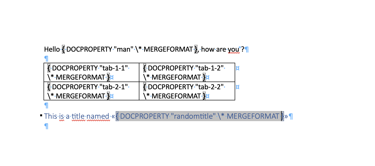
doc <- read_docx("templates/replace-example.docx")
doc <- set_doc_properties(doc, 
  man = "David", 
  `tab-1-1` = "1-1", `tab-1-2` = "1-2",
  `tab-2-1` = "2-1", `tab-2-2` = "2-2",
  randomtitle = "blah blah")
print(doc, target = "static/office/example_doc_properties.docx")

# doconv::docx_update("static/office/example_doc_properties.docx")

static/office/example_doc_properties.docx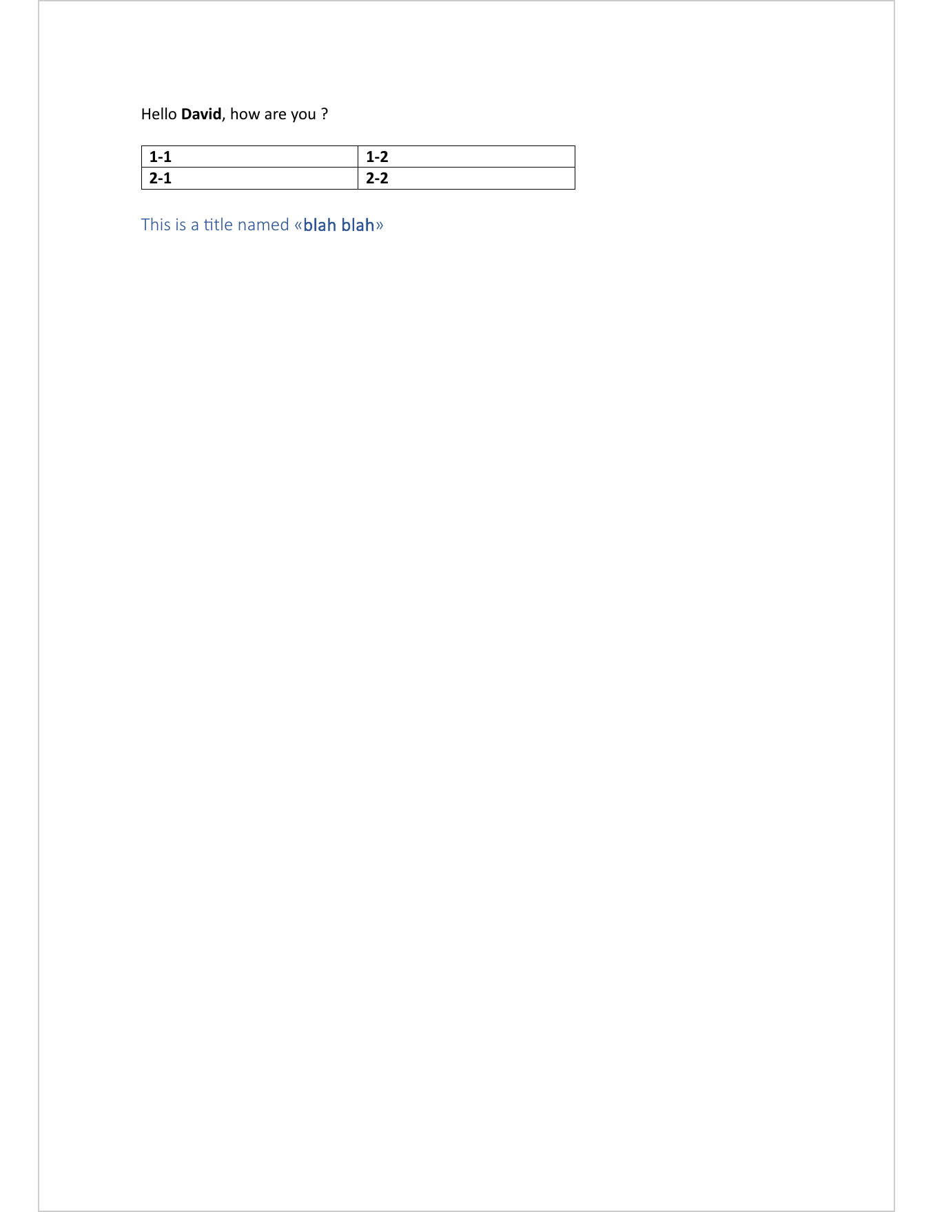

For insertion of complex paragraphs at bookmark level, use:

1. officer::cursor_* functions to position your cursor on a specific block (paragraph or table),
2. and add a block_list() object at this position (using body_add_blocks(pos = "on")).

x <- read_docx(file)
x <- cursor_reach(x, "BLAH BLAH")
x <- body_add_blocks(
  x = x,
  value = block_list(
    fpar(
      "BLIH BLIH",
      fp_p = fp_par(shading.color = "#EFEFEF", text.align = "center"),
      fp_t = fp_text(font.size = 12, font.family = "Calibri", hansi.family = "Calibri")),
    fpar(
      "Blou Blou",
      fp_p = fp_par(shading.color = "red", text.align = "right"),
      fp_t = fp_text(font.size = 10, font.family = "Calibri", hansi.family = "Calibri"))
  ),
  pos = "on")

4.5 Document settings

The functions presented in this section operate at the document level: they do not add content, they configure how content is rendered. They are typically called once, right after read_docx(), before any body_add_*() call.

4.5.1 Managing styles

Word relies heavily on named styles: every paragraph, every run of text can reference a style stored in the document’s style gallery. Styles are the recommended way to apply consistent formatting across a document, and they let Word users re-skin the document later without touching the content itself.

‘officer’ exposes two functions to create or replace styles programmatically:

• docx_set_paragraph_style() for paragraph styles (used by body_add_par(..., style = ...) or by the Table style of body_add_table()),
• docx_set_character_style() for character styles (used by run_wordtext(..., style_id = ...) inside an fpar()).

Both functions add the style if its style_id does not exist yet, and replace it otherwise. Use styles_info() to inspect the styles currently available in the document.

4.5.1.1 Paragraph styles

A paragraph style combines paragraph formatting (alignment, indent, spacing; supplied via fp_p) and default run formatting (font, size, colour, bold / italic; supplied via fp_t). The base_on argument names the existing style the new one inherits from; "Normal" is the usual starting point.

doc <- read_docx()

doc <- docx_set_paragraph_style(
  doc,
  style_id   = "rightaligned",
  style_name = "Right aligned",
  fp_p = fp_par(text.align = "right", padding = 20),
  fp_t = fp_text_lite(bold = TRUE, color = "#1F77B4")
)

doc <- body_add_par(doc,
  value = "A right-aligned, bold, blue paragraph.",
  style = "Right aligned")

print(doc, target = "static/office/example_par_style.docx")

static/office/example_par_style.docx

4.5.1.2 Character styles

A character style carries only run-level formatting (fp_t). It is applied to a portion of a paragraph via run_wordtext() inside an fpar(). base_on must be provided; "Default Paragraph Font" is the conventional base.

doc <- read_docx()

doc <- docx_set_character_style(
  doc,
  style_id   = "highlight",
  style_name = "Highlight",
  base_on    = "Default Paragraph Font",
  fp_t       = fp_text_lite(shading.color = "yellow", color = "black", bold = TRUE)
)

paragraph <- fpar(
  "The word ",
  run_wordtext("highlighted", style_id = "highlight"),
  " stands out."
)

doc <- body_add_fpar(doc, value = paragraph)
print(doc, target = "static/office/example_char_style.docx")

static/office/example_char_style.docx

Styles defined this way become first-class citizens of the document: they appear in Word’s style gallery and downstream users can modify them manually.

4.5.2 General options

docx_set_settings() exposes a handful of document-wide options that are stored in word/settings.xml: default open zoom, default tab stop, hyphenation zone, odd/even headers and footers, first-page header and footer, and Word compatibility mode. These settings are invisible in the document body; a few of them are routine sources of confusion, and the list below is worth keeping in mind before using the function:

• zoom is the zoom level applied when Word opens the file, not a rendering setting. zoom = 1 is 100%, zoom = 2 is 200%. A local Word installation may remember a different zoom from a previous session and mask the effect on your own machine.
• unit governs default_tab_stop and hyphenation_zone. The defaults (0.5 and 0.25) are expressed in inches. Passing unit = "mm" without scaling the numerical values yields a 0.5 mm tab stop, which is almost certainly not what you want.
• compatibility_mode accepts "12", "14" or "15" (default). Lowering it changes the rendering of lists and numbering and should only be used when targeting an older version of Word.
• Odd / even headers and footers are the original motivation for the function; combine it with headers_and_footers() (see the sections chapter) to actually populate the alternating headers.

See ?docx_set_settings for the full argument list.

4.5.3 Document properties

set_doc_properties() writes metadata associated with the file — the same values that Word exposes in File → Info → Properties and that Windows Explorer and enterprise search tools display alongside the document. It handles two distinct kinds of properties:

• Standard properties — title, subject, creator, description, created, and hyperlink_base, passed as named arguments. They are part of the OOXML core / extended properties and are understood by every tool that reads .docx files.
• Custom properties — arbitrary name / value pairs passed via ... (or values). They are used to drive DOCPROPERTY fields in a Word template and are illustrated in the Content Replacement section earlier in this chapter; skip there if that is your primary need.

hyperlink_base is the least intuitive of the standard set: Word uses its value as the base for any relative hyperlink in the document (e.g. a link whose target is docs/report.pdf will resolve against the hyperlink_base path or URL). It is useful for reports that ship with an accompanying folder of external files.

The example below sets a few standard properties on a fresh document:

read_docx() |>
  set_doc_properties(
    title          = "Quarterly report",
    subject        = "Sales overview",
    creator        = "David Gohel",
    description    = "Auto-generated with officer",
    hyperlink_base = "https://example.com/reports/"
  ) |>
  body_add_par("A short document.", style = "Normal") |>
  print(target = "static/office/example_doc_properties_meta.docx")

static/office/example_doc_properties_meta.docx