Chapter 5 officedown for Word
The key features of package ‘officedown’ are :
- Compatibility with the functions of the package ‘officer’ for the production of “runs” and “blocks” of content (text formatting, landscape mode, tables of contents, etc.).
- Ability to use the table styles and list styles defined in the “reference_docx” which serves as a template for the pandoc document.
- The replacement of captions (tables, figures and standard identifiers) by captions containing a Word bookmark that can be used for cross-referencing. Also the replacement of cross-references by cross-references using fields calculated by Word. The syntax conforms to the bookdown cross-reference definition.
- Full support for flextable output, including with outputs containing images and links.
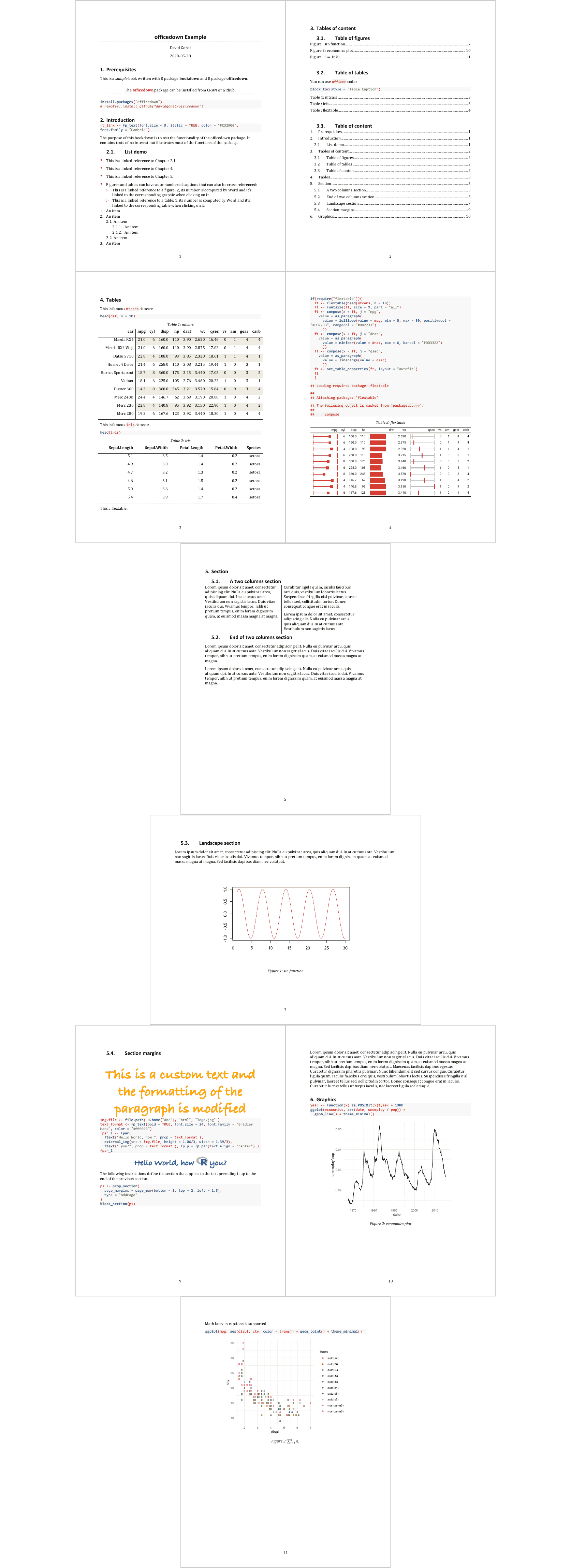
A bookdown is available in the package and can be used as a demo.
dir <- system.file(package = "officedown", "examples", "bookdown")
file.copy(dir, getwd(), recursive = TRUE, overwrite = TRUE)
rmarkdown::render_site("bookdown")
browseURL("bookdown/_book/bookdown.docx")
You should see the following document:
5.1 Automated formatting
The package will automatically perform a set of formatting tasks on the resulting document. The tasks performed are the following:
- Use a Word table template to format all the
data.framethat are printed in the document. - Use two Word list templates (for unordered lists and for ordered lists) to format the set of ordered and ordered lists defined in the R Markdown document.
- Transforming the cross-references and captions defined in the R Markdown document as calculated by Word. It is then easy to copy and paste the content into another document without losing the reference numbers. Captions are also auto-numbered by Word.
The parameters of these transformations are defined in the officedown::rdocx_document function. They can be defined in the YAML header of the R Markdown document.
5.1.1 Tables
The parameter tables is a list that can contain few items to style tables and table captions.
Possible items are the following:
style: the Word stylename to use for tables.layout: ‘autofit’ or ‘fixed’ algorithm.width: value of the preferred width of the table in percent (base 1).caption; caption options, i.e.:style: Word stylename to use for table captions.pre: prefix for numbering chunk (default to “Table”).sep: suffix for numbering chunk (default to “:”).
conditional: a list of named logical values:first_rowandlast_row: apply or remove formatting from the first or last row in the tablefirst_columnandlast_column: apply or remove formatting from the first or last column in the tableno_hbandandno_vband: don’t display odd and even rows or columns with alternating shading for ease of reading.
The default values are the following values:
list(
  style = "Table", layout = "autofit", width = 1,
  caption = list(
    style = "Table Caption", pre = "Table ", sep = ": "),
  conditional = list(
    first_row = TRUE, first_column = FALSE, last_row = FALSE,
    last_column = FALSE, no_hband = FALSE, no_vband = TRUE
  )
)
These values in YAML format are:
output:
  officedown::rdocx_document:
    tables:
      style: Table
      layout: autofit
      width: 1.0
      caption:
       style: Table Caption
       pre: 'Table '
       sep: ': '
      conditional:
       first_row: true
       first_column: false
       last_row: false
       last_column: false
       no_hband: false
       no_vband: true
5.1.2 Plots
The parameter plots is a list that can contain few items to style plots and figure captions.
Possible items are the following:
style: the Word stylename to use for plots.align: alignment of figures in the output document (possible values are ‘left’, ‘right’ and ‘center’).caption; caption options, i.e.:style: Word stylename to use for figure captions.pre: prefix for numbering chunk (default to “Figure”).sep: suffix for numbering chunk (default to “:”).
The default values are the following values:
list(
  style = "Figure",
  align = "center",
  caption = list(
    style = "Image Caption",
    pre = "Figure ", sep = ": "
  )
)
These values in YAML format are:
output:
  officedown::rdocx_document:
    plots:
      style: Normal
      align: center
      caption:
       style: Image Caption
       pre: 'Figure '
       sep: ': '
5.1.3 Lists
The parameter lists is a list that can contain two named items ol.style and
ul.style, values are the stylenames to be used to replace the style of ordered
and unordered lists created by pandoc. If NULL, no replacement is made.
The default values are the following values:
list(ol.style = NULL, ul.style = NULL)These values in YAML format are:
output:
  officedown::rdocx_document:
    lists:
      ol.style: null
      ul.style: null
5.1.4 Page dimensions
You can change the default page dimensions of your document
by setting the values for page_size and page_margins.
# officedown yaml header
output:
  officedown::rdocx_document:
  page_size:
    width: 8.3
    height: 11.7
    orient: "portrait"
  page_margins:
    bottom: 1
    top: 1
    right: 1.25
    left: 1.25
    header: 0.5
    footer: 0.5
    gutter: 0.5
5.2 Default settings
The package is using global settings, used for customization of tables, lists, plots captions and page dimensions.
There is a mechanism to overwrite the defaults with the specified values. This makes it possible not to fill in all the arguments. Thus, a header like the following one is valid:
# officedown yaml header
output:
  officedown::rdocx_document:
    tables:
      caption:
        pre: 'tab. '
5.3 Caption label for figures and tables
Use knitr chunk options fig.cap or tab.cap to specify the label of the
Word caption associated with a table or a figure. If a table, caption will be
added before the table, if a graphic, caption will be added after the
graphic (unless you set chunk option fig.topcaption=TRUE).
---
output: officedown::rdocx_document
---
```{r setup, include=FALSE}
library(officedown)
library(ggplot2)
```
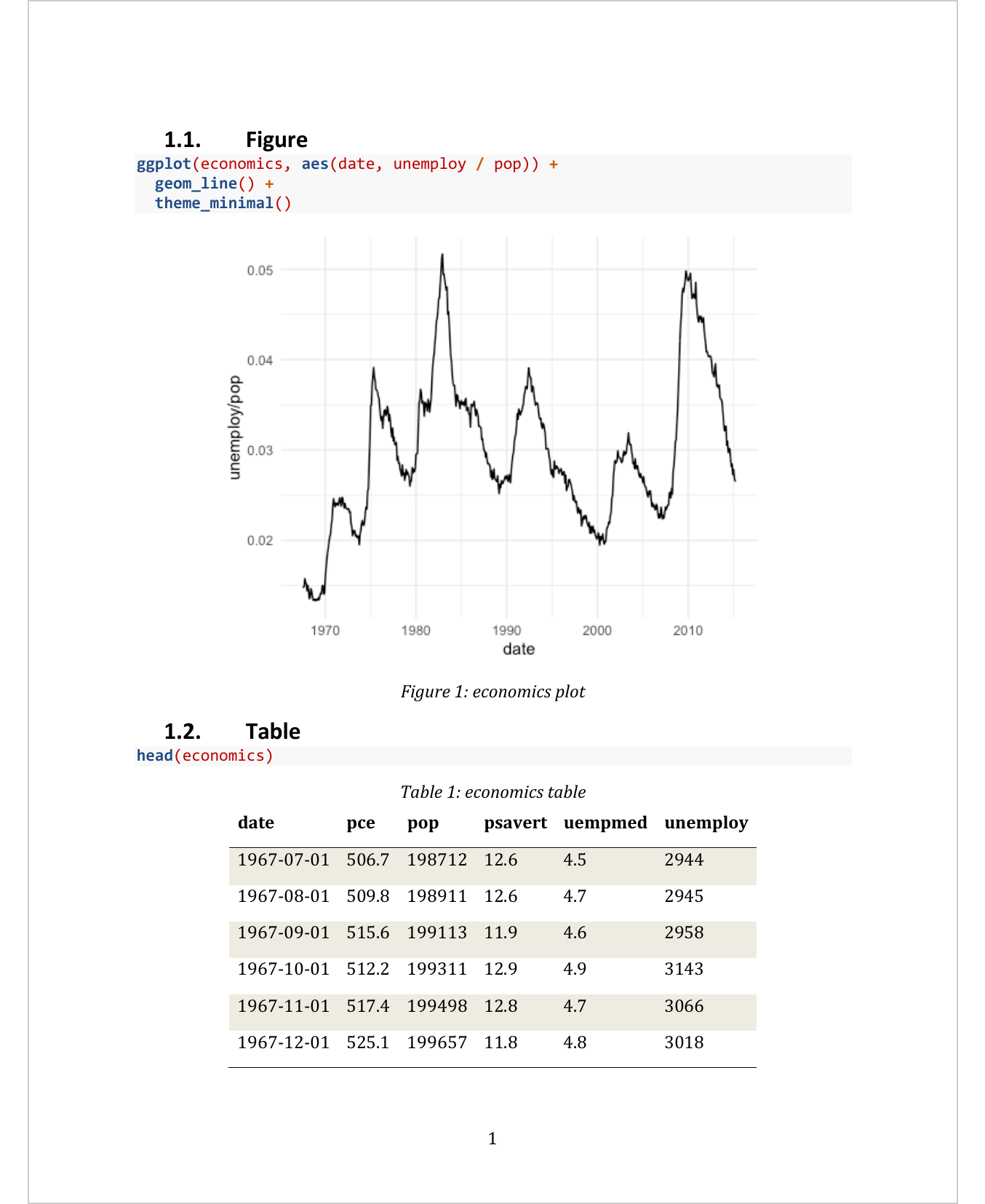
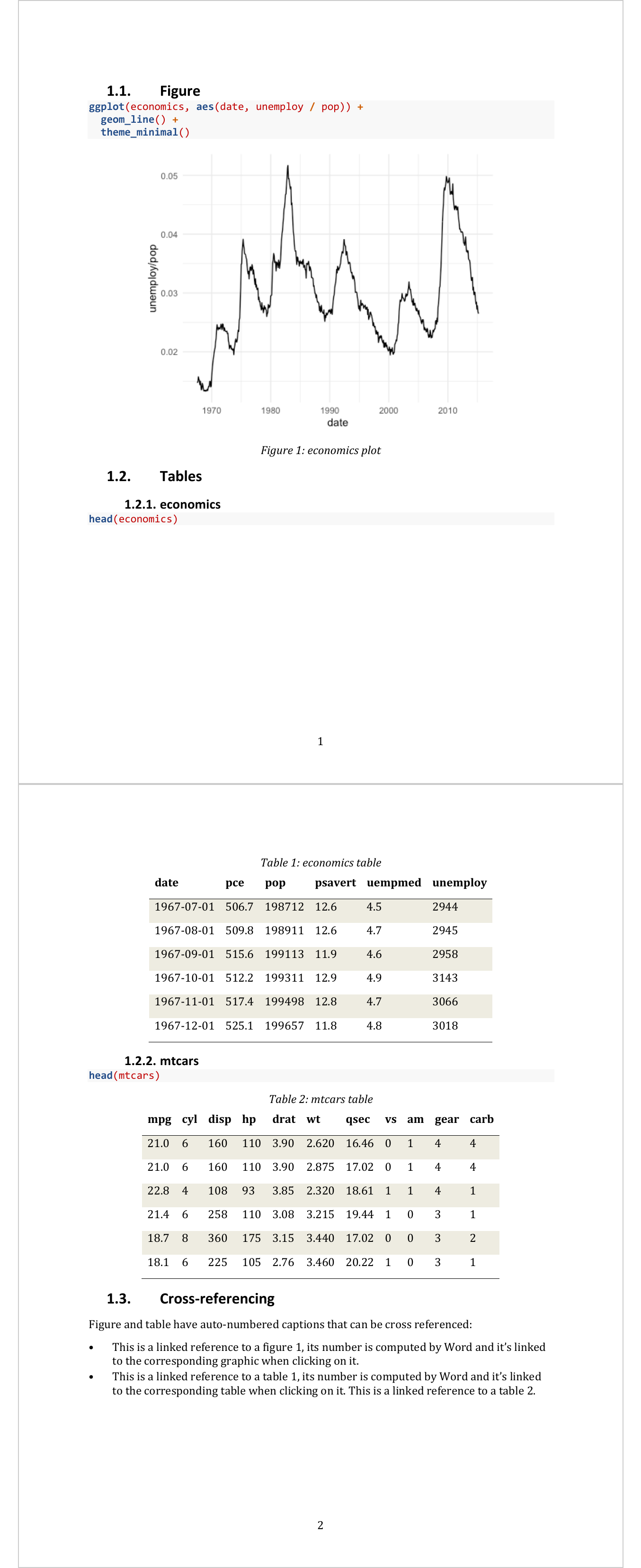
## Figure
```{r fig.cap="economics plot", fig.id = "tsplot", fig.cap.style = "Image Caption"}
ggplot(economics, aes(date, unemploy / pop)) +
geom_line() +
theme_minimal()
```
## Table
```{r tab.cap="economics table", tab.id = "mytab", tab.cap.style = "Table Caption"}
head(economics)
```
Note: you have to update the fields with Word application to reflect the correct caption numbers. See update the fields
Function knitr::opts_chunk$set() or common knitr chunk options can be used to
set the values. Captions for tables and figures can be configured and officedown has special
instructions to manage their values and formats. We have chosen default values
for the options that are common in terms of usage but these values correspond to
the English language. If you are writing in Spanish, German, or another
language, you probably want to change these values to match your language.
---
output: officedown::rdocx_document
---
```{r setup, include=FALSE}
knitr::opts_chunk$set(echo = FALSE)
library(officedown)
```
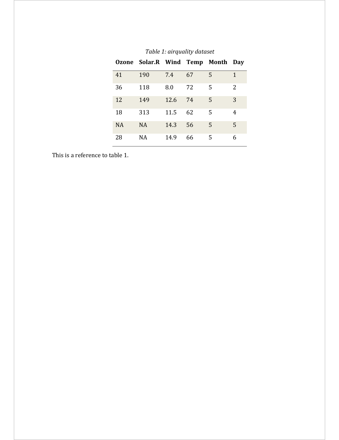
```{r ft.align="center", tab.cap='airquality dataset', tab.id='tab2', label='tab2'}
head(airquality)
```
This is a reference to table \@ref(tab:tab2).
You can change the default values for captions (Word style to use, prefix, separator).
The values to be configured for the tables are the following:
tables:
  caption:
    style: Table Caption
    pre: 'Table '
    sep: ': '
These values can also be altered via the function knitr::opts_chunk$set().
knitr::opts_chunk$set(
  tab.cap.style = "Table Caption",
  tab.cap.pre = "Table ",
  tab.cap.sep = ": ",
  )
The values to be configured for the figures are the following:
plots:
  caption:
    style: Image Caption
    pre: 'Figure '
    sep: ': '
These values can also be altered via the function knitr::opts_chunk$set().
knitr::opts_chunk$set(
  fig.cap.style = "Image Caption",
  fig.cap.pre = "Figure ",
  fig.cap.sep = ": ",
  )
5.4 Cross-references
Cross-referencing is particularly interesting when using {bookdown}. Bookdown
references and captions are not always satisfying some organizations
requirements that impose usage of computed numbered captions and references to
them for Word documents. ‘officedown’ bring this feature: caption are autonumbered
and a bookmark is set on the chunk containing the number; cross-references are Word
references hyperlinked to the captions they are related to.
The functionality will allow the editing of Word documents produced with respect of different references or numbered captions. This is particulary useful when the document is modified in its structure (chapters moved, graphics added manually) or integrated into another Word document.
---
output: officedown::rdocx_document
---

```{r setup, include=FALSE}
library(officedown)
library(ggplot2)
```

## Figure

```{r fig.cap="economics plot", fig.id = "tsplot", fig.cap.style = "Image Caption"}
ggplot(economics, aes(date, unemploy / pop)) +
  geom_line() +
  theme_minimal()
```

## Tables

### economics

```{r tab.cap="economics table", tab.id = "mytab", tab.cap.style = "Table Caption"}
head(economics)
```

### mtcars

```{r tab.cap="mtcars table", tab.id = "mtcars", tab.cap.style = "Table Caption"}
head(mtcars)
```

## Cross-referencing

Figure and table have auto-numbered captions that can be cross referenced:

* This is a linked reference to a figure \@ref(fig:tsplot), its number is computed by Word
and it's linked to the corresponding graphic when clicking on it.
* This is a linked reference to a table \@ref(tab:mytab), its number is computed by Word
and it's linked to the corresponding table when clicking on it. This is a linked reference to
a table \@ref(tab:mtcars).
To refer to simple document id, use syntax \@ref(an_id):
5.4.1 Custom cross-reference
officedown has been implemented with the intention of supporting the bookdown syntax as much as possible. The addition of cross-references will generate a numbered reference (the caption number of the graph or table).
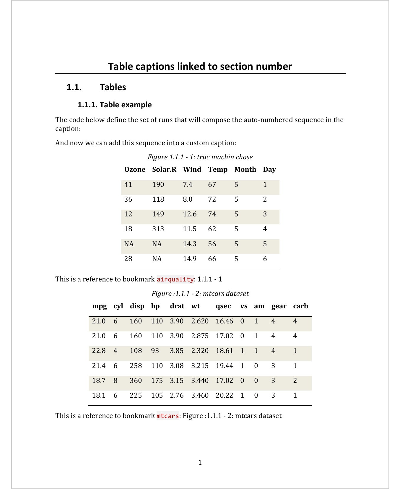
If you want a different cross-reference, then you will have to manually recompose the caption. The following example shows how to add captions that also contain the number of the chapter that contains it.
---
title: "Table captions linked to section number"
output: officedown::rdocx_document
---

```{r setup, include=FALSE}
knitr::opts_chunk$set(echo = FALSE)
library(officedown)
library(officer)
```

## Tables

### Table example

The code below define the set of runs that will compose the auto-numbered sequence in the caption:

```{r}
runs <- list(
  run_word_field("STYLEREF 3 \\s"),
  ftext(" - "),
  run_autonum(seq_id = "tab", pre_label = "", post_label = "")
)
```

And now we can add this sequence into a custom caption:

::: {custom-style="Table Caption"}


Figure `r run_bookmark("airquality", runs)`: truc machin chose


:::

```{r}
head(airquality)
```

This is a reference to bookmark `airquality`: `r run_reference(id = "airquality")`

```{r}
runs_0 <- list(ftext("Figure :"))
runs_p <- list(ftext(": mtcars dataset"))
runs <- append(runs_0, runs)
runs <- append(runs, runs_p)
```

::: {custom-style="Table Caption"}


`r run_bookmark("mtcars", runs)`


:::

```{r}
head(mtcars)
```

This is a reference to bookmark `mtcars`: `r run_reference(id = "mtcars")`
5.5 Paragraphs, tables and TOC
Paragraphs defined with the fpar() function as well as many other objects from the officer package can be used within a R Markdown document.
5.5.1 Formatted paragraphs
Objects produced by function fpar can be integrated into the final document:
---
output: officedown::rdocx_document
---

```{r setup, include=FALSE}
knitr::opts_chunk$set(echo = TRUE, fig.cap = TRUE)
library(officedown)
library(officer)
```

```{r echo=FALSE}
img.file <- file.path( R.home("doc"), "html", "logo.jpg" )

bold_face <- shortcuts$fp_bold(font.size = 20)
bold_redface <- update(bold_face, color = "red")
fpar_1 <- fpar(
  ftext("How ", prop = bold_redface ),
  external_img(src = img.file, height = 1.06/2, width = 1.39/2),
  ftext(" you?", prop = bold_face ) )
fpar_1
```

5.5.2 Add Word captions
Objects produced by function block_caption can be added as in the following example.
---
output: officedown::rdocx_document
---

```{r setup, include=FALSE}
knitr::opts_chunk$set(echo = TRUE, fig.cap = TRUE)
library(officedown)
library(officer)
```

```{r echo=FALSE}
head(airquality)
run_num <- run_autonum(seq_id = "tab", pre_label = "tab. ", bkm = "iris_table")
block_caption("iris table",
              style = "Table Caption",
              autonum = run_num )
```
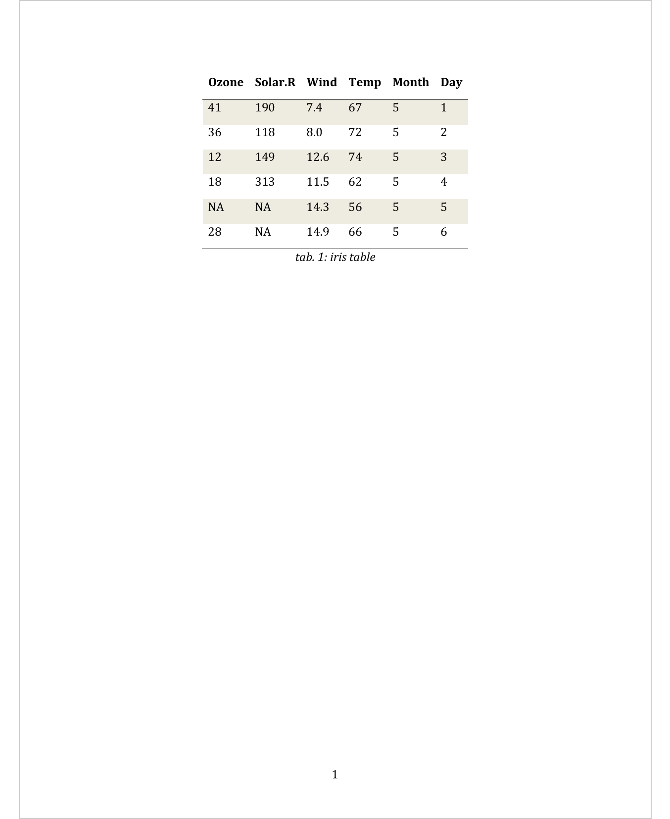
The bookmark iris_table has been added around the number of the caption, this number
is automatiically computed by Word and can be re-used ; as a reference to be used in another
paragraph most of the time.
read_docx("static/rmd/block_caption.docx") |>
  docx_bookmarks()
# [1] "iris_table"5.5.3 Tables
The subject of tables is vast and here we are only talking about simple tables for Word. For complex formatting, the ‘flextable’ package is preferable.
5.5.4 TOC
A TOC (Table of Contents) is a Word computed field, table of contents is built by Word. The TOC field will collect entries using heading styles or another specified style.
Note: you have to update the fields with Word application to reflect the correct page numbers. See update the fields
---
output: officedown::rdocx_document
---
```{r setup, include=FALSE}
library(officedown)
library(officer)
library(ggplot2)
```
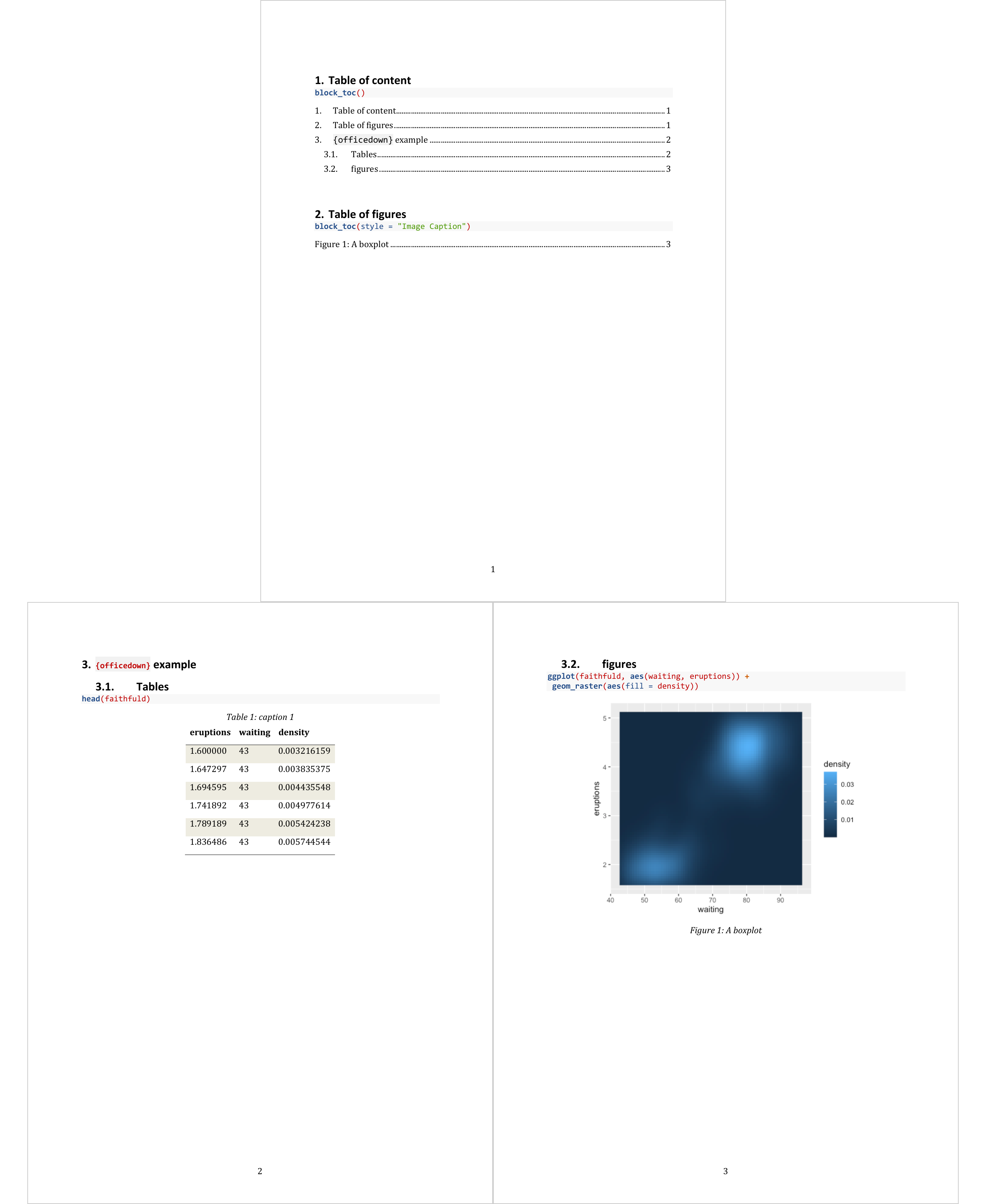
# Table of content
```{r}
block_toc()
```
# Table of figures
```{r}
block_toc(style = "Image Caption")
```
\newpage
# `'officedown'` example
## Tables
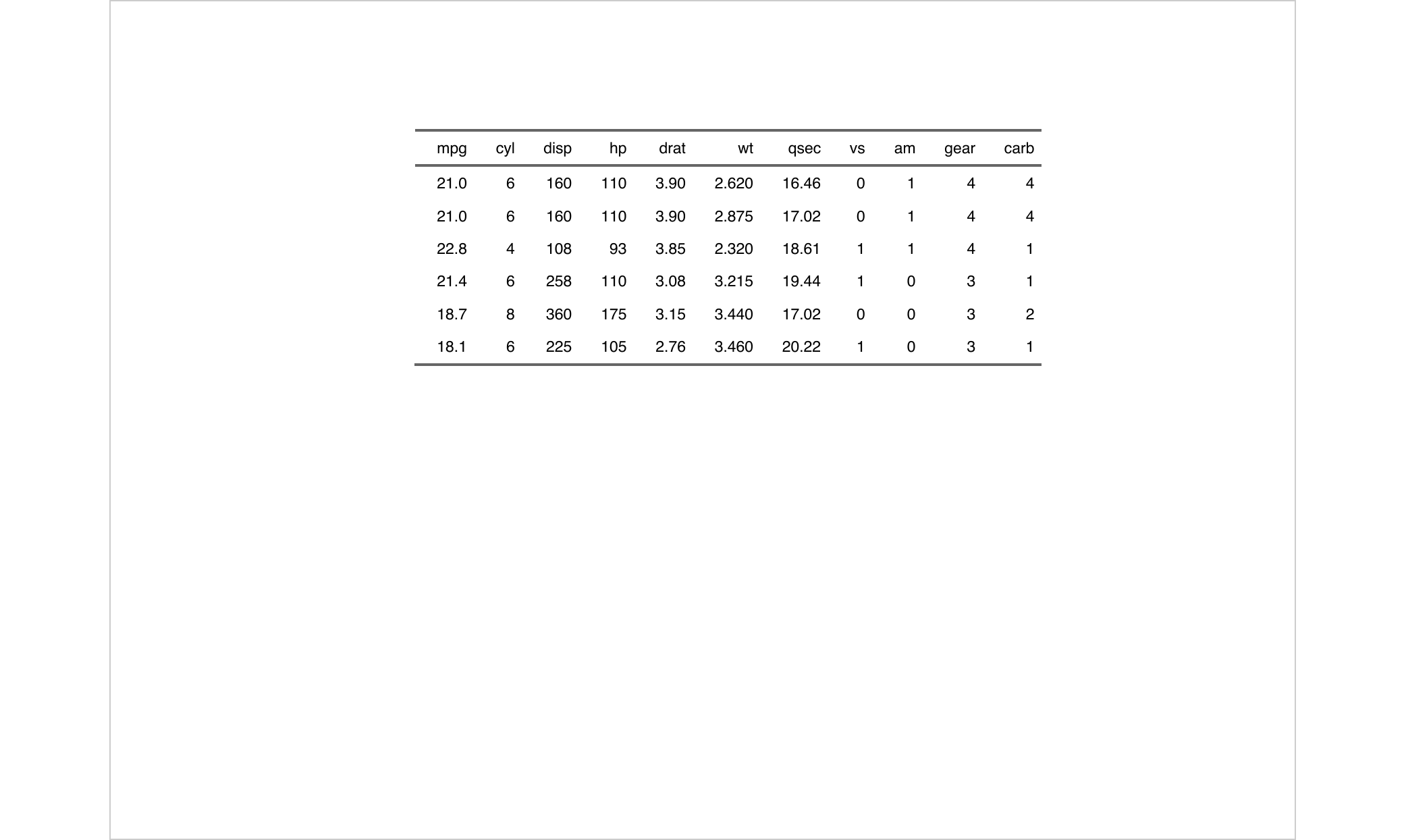
```{r tab.cap="caption 1", tab.id="faithfuld"}
head(faithfuld)
```
\newpage
## figures
```{r fig.cap="A boxplot", fig.id = "faithfuld-plot"}
ggplot(faithfuld, aes(waiting, eruptions)) +
geom_raster(aes(fill = density))
```
5.5.5 Lists of Figures and Tables
You can list and organize the figures or tables in a Word document by creating a table of figures, much like a table of contents.
5.5.5.1 Using stylename
R Markdown uses the Word paragraph style “Image Caption” for graphic captions. To my knowledge, there is no official feature for table captions and therefore no style associated with table captions. Word, on the other hand, only uses a paragraph style called “Caption” whether the caption is relative to a graph, a table or an equation. Note that this style name is specific to each country.
The choice that has been made with officedown is to let you apply
one or different styles for table and graph captions. Default style for graph
captions is “Image Caption” and default style for table captions is “Table Caption”
(which is also available in R Markdown (and pandoc) Word template.
Create a list of figures with function block_toc or by using
officedown chunk <!---BLOCK_TOC{...}--->
If you used two different styles for table and figures captions, use block_toc with
argument style set to the caption style name.
block_toc(style = "Table Caption")OR
<!---BLOCK_TOC{style: "Table Caption"}--->
5.5.5.2 Using sequence identifier
You might have to (or want to) use only one single style for table and graphic captions and need to generate one table of contents for tables and one for charts.
In that case use block_toc with argument seq_id set by default to tab for
table captions and fig for figure captions.
block_toc(seq_id = "tab")OR
<!---BLOCK_TOC{seq_id: "fig"}--->
5.5.6 Embbed Word document
You can pour the content of a docx file in the resulting docx generated by the main R Markdown document.
---
output: officedown::rdocx_document
---
```{r setup, include=FALSE}
library(officedown)
library(officer)
```
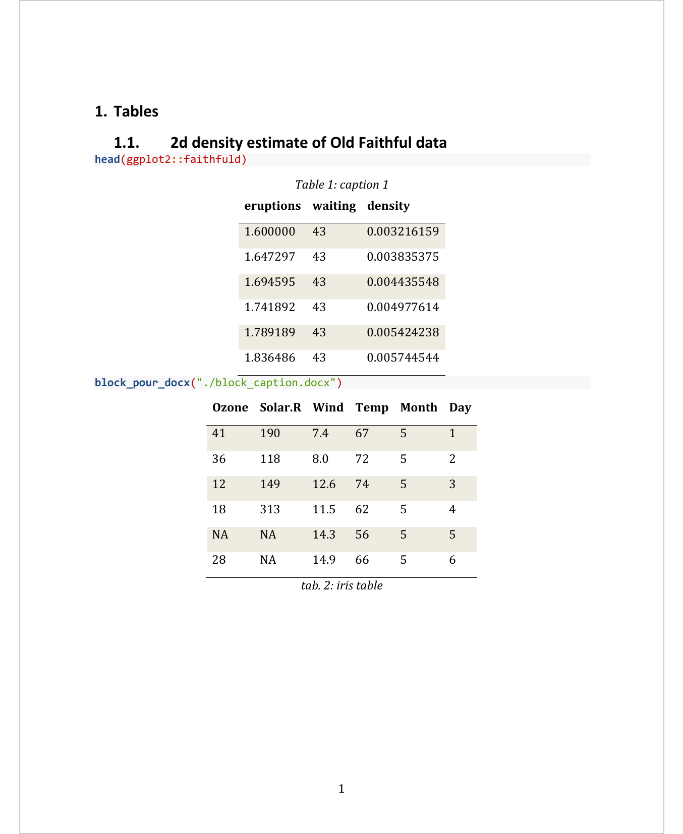
# Tables
## 2d density estimate of Old Faithful data
```{r tab.cap="caption 1", tab.id="faithfuld"}
head(ggplot2::faithfuld)
```
```{r}
block_pour_docx("./block_caption.docx")
```
5.6 Insert sections
A section affects preceding paragraphs or tables (see Word Sections).
Usually, starting with a continous section and ending with the section you defined is enough.
To format your content in a section, you can use the section tags or
define the section with the block_section function, which takes an object
returned by the prop_section function. It is prop_section() that allows
you to define the properties of your section.
5.6.1 Tags for sections
Tags (as HTML comments) have been designed to be less verbose and easier to use; for landscape pages, for multi-columns sections and for tables of contents.
---
output: officedown::rdocx_document
---

```{r setup, include=FALSE}
knitr::opts_chunk$set(echo = TRUE, fig.cap = TRUE)
library(officedown)
```

The following will be transformed as a table of content:

<!---BLOCK_TOC--->

And the following will pour the content of an external docx file into the produced document:

<!---BLOCK_POUR_DOCX{docx_file: 'path/to/docx'}--->
The parameters are defined in a yaml string. Each item in the list is a list of key/value pairs defined with
key: valueform (the colon must be followed by a space).
These tags need to be used in pairs:
landscape orientation
| Tag name | R function |
|---|---|
| BLOCK_LANDSCAPE_START | block_section(prop_section(type = “continuous”)) |
| BLOCK_LANDSCAPE_STOP | block_section(prop_section(page_size = page_size(orient = “landscape”))) |
The type of page break is set to oddPage.
section with columns
| Tag name | R function |
|---|---|
| BLOCK_MULTICOL_START | block_section(prop_section(type = “continuous”)) |
| BLOCK_MULTICOL_STOP | block_section(prop_section(section_columns = section_columns(widths = c(4.75, 4.75)))) |
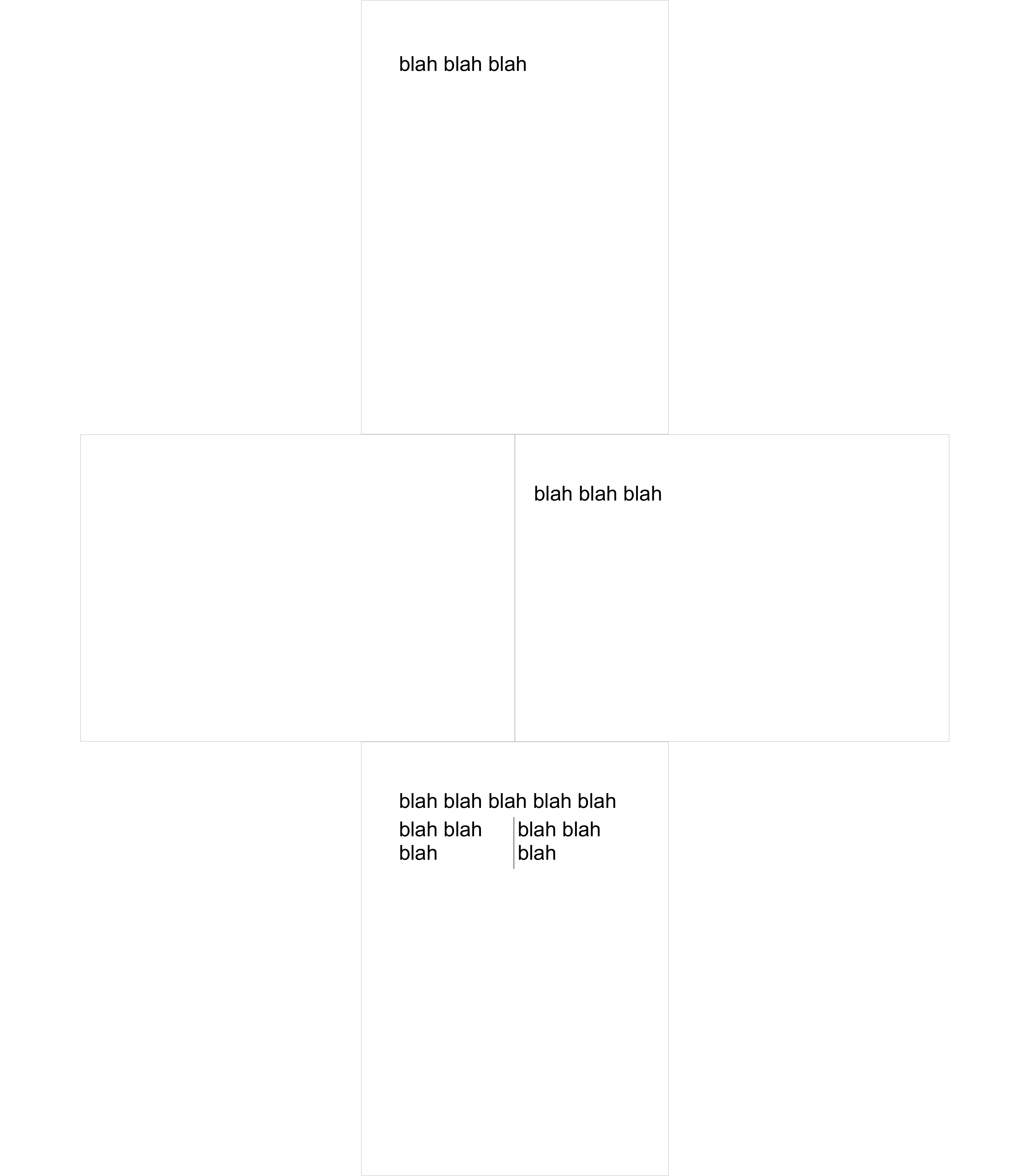
The following R Markdown document illustrate the tags:
---
output: officedown::rdocx_document
---

```{r setup, include=FALSE}
knitr::opts_chunk$set(echo = TRUE, fig.cap = TRUE)
library(officedown)
library(officer)
ft <- fp_text(font.size = 40)
```

`r ftext("blah blah blah", ft)`

<!---BLOCK_LANDSCAPE_START--->

`r ftext("blah blah blah", ft)`

<!---BLOCK_LANDSCAPE_STOP--->

`r ftext("blah blah blah blah blah", ft)`

<!---BLOCK_MULTICOL_START--->

`r ftext("blah blah blah", ft)`

`r officer::run_columnbreak()``r ftext("blah blah blah", ft)`

<!---BLOCK_MULTICOL_STOP{widths: [3,3], space: 0.2, sep: true}--->
5.6.2 Function block_section
If the default settings associated with the tags don’t satisfy your needs, you can
define a section ending with a call to function block_section within a knitr
R chunk.
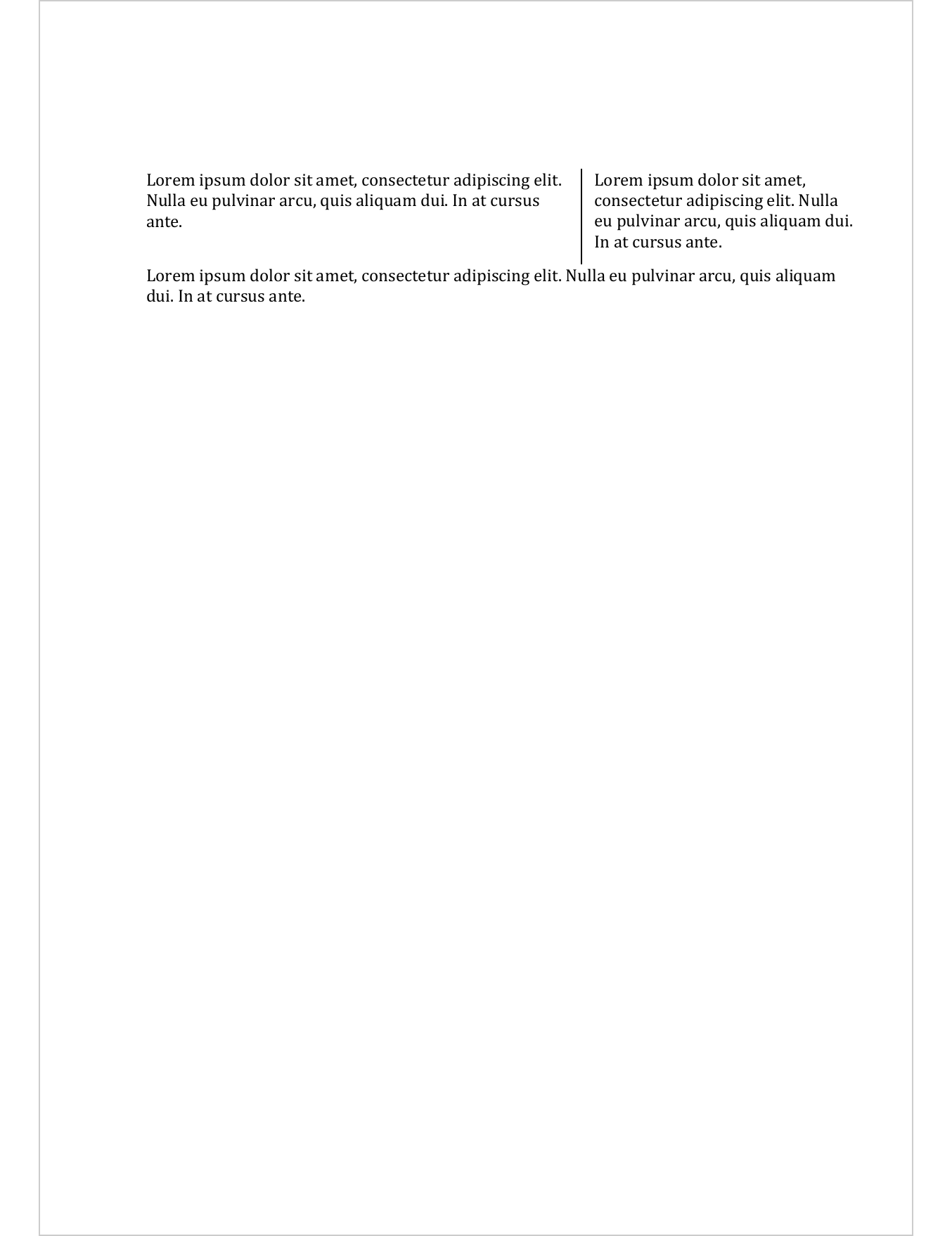
Here is an example with a two column section:
---
output: officedown::rdocx_document
---

```{r setup, include=FALSE}
knitr::opts_chunk$set(echo = FALSE)
library(officedown)
library(officer)
```

```{r}
block_section(prop_section(type = "continuous"))
```

Lorem ipsum dolor sit amet, consectetur adipiscing elit. Nulla eu pulvinar arcu,
quis aliquam dui. In at cursus ante.

`r run_columnbreak()`Lorem ipsum dolor sit amet, consectetur adipiscing elit. Nulla eu pulvinar arcu,
quis aliquam dui. In at cursus ante.

```{r}
block_section(
  prop_section(
    section_columns = section_columns(
      widths = c(4,2.5), space = .25, sep = TRUE),
    type = "continuous"))
```

Lorem ipsum dolor sit amet, consectetur adipiscing elit. Nulla eu pulvinar arcu,
quis aliquam dui. In at cursus ante.
Here is an example with a landscape section (the first page only can be seen on the screenshot):
---
output: officedown::rdocx_document
---

```{r setup, include=FALSE}
knitr::opts_chunk$set(echo = FALSE)
library(officedown)
library(officer)
library(flextable)
```

```{r}
qflextable(head(mtcars))
```

```{r}
block_section(
  prop_section(
    page_size = page_size(orient = "landscape"),
    type = "continuous"
  )
)
```
5.7 Insert formatted texts
To add a formatted run in your document use knitr Inline Code syntax. By enclosing an ‘officer’ run code with “r”, you
can add formatted chunk at any location in your R Markdown
document.
The following is a simple example of inserting a text associated with some text formatting properties.
---
output: officedown::rdocx_document
---

```{r setup, include=FALSE}
knitr::opts_chunk$set(echo = FALSE)
library(officedown)
library(officer)

ft_example <- fp_text_lite(
  color = "red", bold = TRUE, font.size = 50)
```

This is some text made with `r ftext("officedown", ft_example)`.
There are many run_* functions dedicated to Word output:
run_autonum(),external_img(),ftext(),hyperlink_ftext(),run_bookmark(),run_columnbreak(),run_footnoteref(),run_footnote(),run_linebreak(),run_pagebreak(),run_reference(),run_word_field()
The following is illustrating some of them:
5.7.1 Reference a bookmarked text
---
output: officedown::rdocx_document
---

```{r setup, include=FALSE}
knitr::opts_chunk$set(echo = FALSE, fig.cap = TRUE)
library(officedown)
library(officer)
ft_obj1 <- fp_text_lite(color = "green", bold = TRUE)
ft_obj2 <- fp_text_lite(color = "red", bold = TRUE)
```

## Custom caption

This is a text with an associated format and this text is bookmarked as "par1":

On dit `r run_bookmark("par1", ftext("pain au chocolat", ft_obj1))`! On ne dit pas `r ftext("chocolatine", ft_obj2)`.

## References

This is a reference to `r run_reference(id = "par1", prop = ft_obj1)`.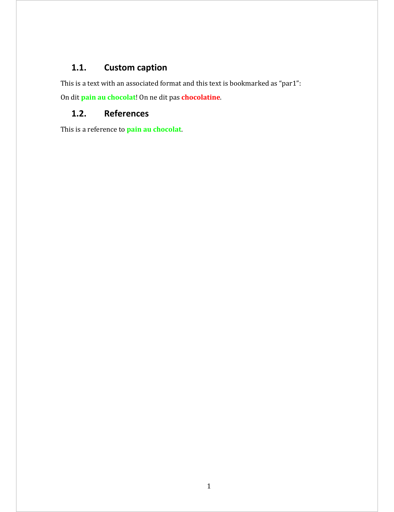
5.7.2 Custom caption
---
output: officedown::rdocx_document
---

```{r setup, include=FALSE}
knitr::opts_chunk$set(echo = FALSE)
library(officedown)
library(officer)

ft_example <- fp_text_lite(
  color = "red", bold = TRUE)
srcfile <- file.path( R.home("doc"), "html", "logo.jpg" )
extimg <- external_img(src = srcfile, height = 1.06/5, width = 1.39/5)
```

Blah blah blah blah blah blah blah blah blah blah blah blah blah blah blah blah
blah blah blah blah blah blah blah blah blah blah blah blah blah blah blah blah
blah blah blah blah blah blah blah blah blah blah blah blah blah blah blah blah
blah blah blah blah blah blah blah blah blah blah blah blah blah blah blah blah
blah blah blah blah blah blah blah blah blah blah blah blah blah blah blah blah
blah blah blah blah blah blah blah blah blah blah blah blah blah blah blah blah
blah blah blah blah.

<caption>
`r run_autonum(seq_id = 'fig', bkm = 'faithful-plot', pre_label = "Figure ", prop = ft_example, bkm_all = TRUE)`
Faithfuld plot `r extimg`
</caption>

```{r}
plot(faithful)
```

Blah blah blah blah blah blah blah blah blah blah blah blah blah blah blah blah
blah blah blah blah blah blah blah blah blah blah blah blah blah blah blah blah
blah blah blah blah blah blah blah blah blah blah blah blah blah blah blah blah
blah blah blah blah blah blah blah blah blah blah blah blah blah blah blah blah
blah blah blah blah blah blah blah blah blah blah blah blah blah blah blah blah
blah blah blah blah blah blah blah blah blah blah blah blah blah blah blah blah
blah blah blah blah.

This is a reference to `r run_reference(id = "faithful-plot", prop = ft_example)`.

Blah blah blah blah blah blah blah blah blah blah blah blah blah blah blah blah
blah blah blah blah blah blah blah blah blah blah blah blah blah blah blah blah
blah blah blah blah blah blah blah blah blah blah blah blah blah blah blah blah
blah blah blah blah blah blah blah blah blah blah blah blah blah blah blah blah
blah blah blah blah blah blah blah blah blah blah blah blah blah blah blah blah
blah blah blah blah blah blah blah blah blah blah blah blah blah blah blah blah
blah blah blah blah.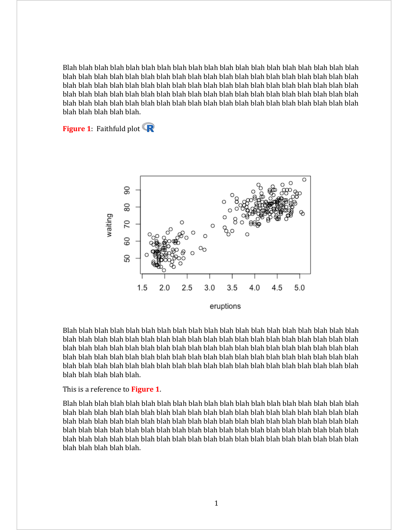
5.7.3 Word Computed field
---
output: officedown::rdocx_document
---
```{r setup, include=FALSE}
knitr::opts_chunk$set(echo = FALSE, fig.cap = TRUE)
library(officedown)
library(officer)
```
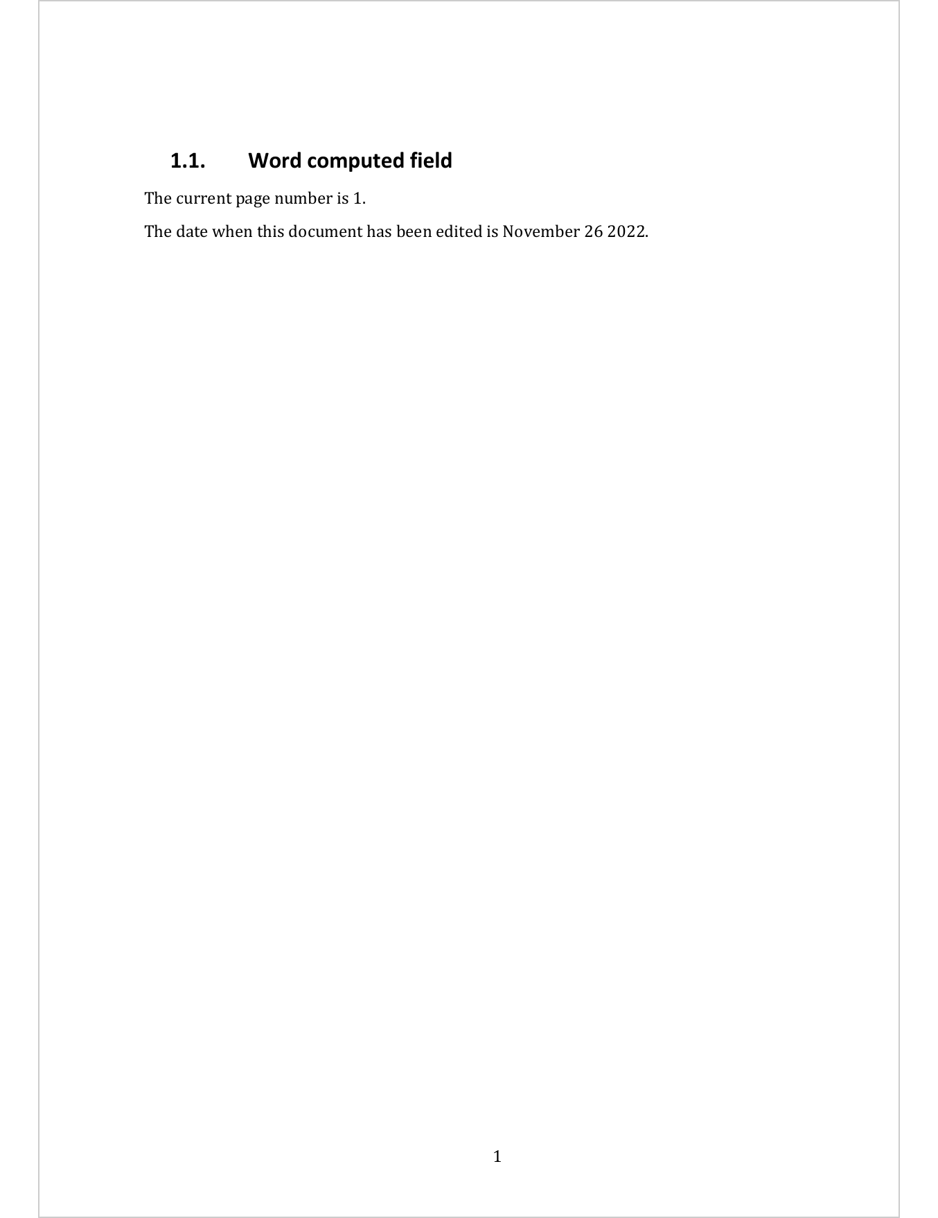
## Word computed field
The current page number is `r run_word_field(field = "PAGE \\* MERGEFORMAT")`.
The date when this document has been edited is `r run_word_field(field = "Date \\@ \"MMMM d yyyy\"")`.